7.3. Using Support Vector Machines for classification tasks
In this section we illustrate the basic idea behind a kind of linear classifier called an Support Vector Machine (SVM). We demonstrate the idea by cooking up a set of points that creates a classification problem with a very easy solution.
Let’s do some imports.
import numpy as np
import pandas as pd
import sklearn
import sklearn.datasets as ds
import sklearn.cross_validation as cv
import sklearn.grid_search as gs
import sklearn.svm as svm
import matplotlib as mpl
import matplotlib.pyplot as plt
%matplotlib inline
We generate a scattering of 2D points X and assign a binary label y according to a linear operation on the coordinates.
X = np.random.randn(200, 2)
y = X[:, 0] + X[:, 1] > 1
The label is True (“positive”) if the sum of the two coordinates is greater than 1; otherwise False. This is an easy linear problem.
print X.shape, X[0,0], X[0,1]
print y[0]
(200, 2)
0.337414510071 -1.94889565504
False
X is a 200x2 array. The values of the coordinates for the first item in X, X[0,:], are shown, as well as the label, computed by the rule given above, X belongs in the False category because the sum of its two coordinates is less then 1.
We now fit a linear Support Vector Classifier (SVC). This classifier tries to find a line (a line here, more generally a hyperplane) that separates the True labels from the False labels. Otherwise put, we train the classifier. The output of training is a decision function that tells us how close to the line we are (close to the boundary means a low-confidence decision). Positive decision values mean True, Negative decision values mean False.
est = svm.LinearSVC()
est.fit(X, y);
For visualization purposes only (specifically, to use the contour plot below), we manipulate the data into a “mesh grid” shape. We’re going to plot decisions for 250,000 points in a 250x250 rectangle. To do that we’ll store the decision results Z in an array with the same 250x250 meshgrid shape.
# We generate a grid in the square [-3,3 ]^2.
xx, yy = np.meshgrid(np.linspace(-3, 3, 500),
                     np.linspace(-3, 3, 500))

# Flatten the meshgrid so we can apply the decision function
Z = est.decision_function(np.c_[xx.ravel(), yy.ravel()])
# Put the results back in the right 250x250 shape
Z = Z.reshape(xx.shape)
print xx.shape,Z.shape
print 'Two sample points in the grid, first the x-ordinates, then the y'

print xx[0,0], xx[1,0], xx[0,1],xx[1,1]
print yy[0,0], yy[1,0], yy[0,1],yy[1,1]

print 'Now the value of the decision function for those points.  It will be a high positive number for high-confidence positive decisions.'
print 'It will have a low absolute value (near 0) for low-confidence decisions.'
print 'It will change each time you run this notebook, because a new set of random points is chosen on each run.'
print Z[0,0], Z[0,1], Z[1,0], Z[1,1]
print 'The real shape of the data in table form is 250000 2 D points, a 250000x2 array'
print np.c_[xx.ravel(),yy.ravel()].shape
(500, 500) (500, 500)
Two sample points in the grid, first the x-ordinates, then the y
-3.0 -3.0 -2.9879759519 -2.9879759519
-3.0 -2.9879759519 -3.0 -2.9879759519
Now the value of the decision function for those points. It will be a high positive number for high-confidence positive decisions.
It will have a low absolute value (near 0) for low-confidence decisions.
It will change each time you run this code, because a new set of random points is chosen on each run.
-14.1720860306 -14.1480419983 -14.147005555 -14.1229615227
The “flat” shape of the data in table form is 250000 2 D points, a 250000x2 array
(250000, 2)
We define a function that displays the boundaries and decision function
of a trained classifier. The scatter function displays our points on
the 2D grid we defined. We show the regions of the grid where the
decision surface Z has the highest values in dark blue with
imshow, and we show the place where Z is 0 with the contour
function, instructing it to draw a black line along the pointss where
z=0. The scatter function assigns a color to points as well.
Those for which the class value (y) is 1 are dark; those with class
value 0 are light (open circles). We draw dashed axis lines with the
axhline and axvline commands.
# This plotting function takes an SVM estimator as input.
def plot_decision_function(est):
    xx, yy = np.meshgrid(np.linspace(-3, 3, 500),
                         np.linspace(-3, 3, 500))
    # We evaluate the decision function on the grid.
    Z = est.decision_function(np.c_[xx.ravel(), yy.ravel()])
    Z = Z.reshape(xx.shape)
    cmap = plt.cm.Blues
    # We display the decision function on the grid.
    plt.figure(figsize=(5,5));
    plt.imshow(Z,
                extent=(xx.min(), xx.max(), yy.min(), yy.max()),
                aspect='auto', origin='lower', cmap=cmap);
    # We display the boundary where Z = 0
    plt.contour(xx, yy, Z, levels=[0], linewidths=2,
                colors='k');
    # All point colors c fall in the interval .5<=c<=1.0 on the blue colormap. We color the true points darker blue.
    plt.scatter(X[:, 0], X[:, 1], s=30, c=.5+.5*y, lw=1,
                cmap=cmap, vmin=0, vmax=1);
    plt.axhline(0, color='k', ls='--');
    plt.axvline(0, color='k', ls='--');
    plt.xticks(());
    plt.yticks(());
    plt.axis([-3, 3, -3, 3]);
Let’s take a look at the classification results with the linear SVC.
plot_decision_function(est);
plt.title("Linearly separable, linear SVC");
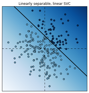
The linear SVC tried to separate the points with a line and it did a pretty good job.
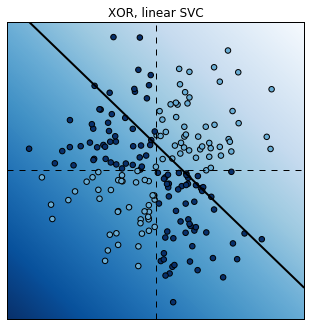
We now modify the labels with a XOR function. A point’s label is 1 if the coordinates have different signs. This classification is not linearly separable. Therefore, a linear SVC fails completely.
y = np.logical_xor(X[:, 0] > 0, X[:, 1] > 0)
# We train the classifier.
est = gs.GridSearchCV(svm.LinearSVC(),
                      {'C': np.logspace(-3., 3., 10)});
est.fit(X, y);
print("Score: {0:.1f}".format(
      cv.cross_val_score(est, X, y).mean()))
# Plot the decision function.
plot_decision_function(est);
plt.title("XOR, linear SVC");
Score: 0.6
Fortunately, it is possible to use non-linear SVCs by using non-linear
kernels. Kernels specify a non-linear transformation of the points
into a higher-dimensional space. Transformed points in this space are
assumed to be more linearly separable, although they are not necessarily
in the original space. By default, the SVC classifier in
scikit-learn uses the Radial Basis Function (RBF) kernel.
y = np.logical_xor(X[:, 0] > 0, X[:, 1] > 0)
est = gs.GridSearchCV(svm.SVC(),
                      {'C': np.logspace(-3., 3., 10),
                    'gamma': np.logspace(-3., 3., 10)});
est.fit(X, y);
print("Score: {0:.3f}".format(
      cv.cross_val_score(est, X, y).mean()))
plot_decision_function(est.best_estimator_);
plt.title("XOR, non-linear SVC");
Score: 0.945
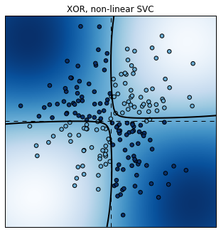
This time, the non-linear SVC does a pretty good job at classifying these non-linearly separable points.
Now transforming the data in some way in order to make it easier to classify is an idea we’ve already seen. We did this to Iris data to find a 2D representation that we could classify with high accuracy and was still easy to visualize. The difference is that in that case we did dimensionality reduction. In this case we increase the dimensionality. Now at first blush that seems nuts, but if we know of some structural relationship between the features, sometimes the added dimension can create a separation between features that wasn’t there before, and in the higher dimension space, a hyperplane can separate classes that are inseparable at lower dimensions. That’s what has happened here.
The material in this section was adapted from
IPython Cookbook, by Cyrille Rossant, Packt Publishing, 2014 (500 pages).