9.6. Dimensionality reduction

Most social science data is high-dimensional. That is, we are looking at many variables at once. Visualization of high-dimensional datasets can be hard. While data in two or three dimensions can be plotted to show the inherent structure of the data, equivalent high-dimensional plots can be much harder to understand. As we will show with House votes example below, reducing the dimensionality of the data can be very helpful in finding its structure.

The simplest way to accomplish this dimensionality reduction is by taking a random projection of the data. Though this sometimes allows some degree of understanding of the data structure, the randomness of the choice may well lose the more interesting information within the data. In the figure below, due to Eamonn Keogh and Jessica Lin, a set of data points in 3 dimensions is projected into 2 dimensions along 3 different axes, yielding three very different shapes. Let’s say the triangle captures the structure you are interested in the data. But each projection yields a very different picture.

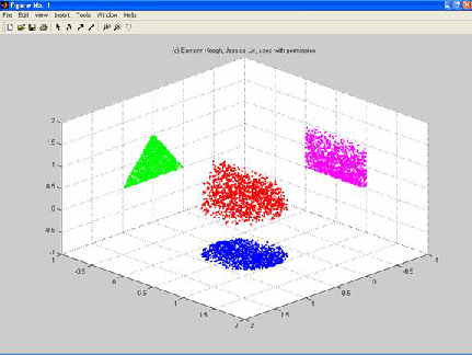
How will you know which projection to use? It may not be practical to do all possible projections when there are thousands of variables; nor is it necessarily the case the that you will know which picture is the right one just by looking at it. Finally, projecting is just selecting a few variables and ignoring all the others. There are techniques of dimensionality reduction that don’t work that way. Instead we try to find a single new dimension that captures as much information as possible from multiple dimensions in the original data set.

Many of the most important dimensionality reduction techniques are linear. That is, they involve linear equations that boil M numbers down to N numbers (N < M). These include Principal Component Analysis (PCA), Independent Component Analysis, Linear Discriminant Analysis, and others. These algorithms define specific ways to choose an “interesting” linear projection of the data. They can and do miss important non-linear structure in the data, but they can be very useful. We will look at one example of such a technique, Latent Semantic Analysis (LSA, which is very closely related to PCA) [1] .

9.6.1. An example

Below we see a simple two dimensional visualization of House of Representatives voting patterns, achieved by LSA. Essentially what happens is that we reduce the voting pattern from 16 dimensions to 2, and in doing so, we effectively cluster representatioves together in a way that seems to capture party affiliations (represented by color).

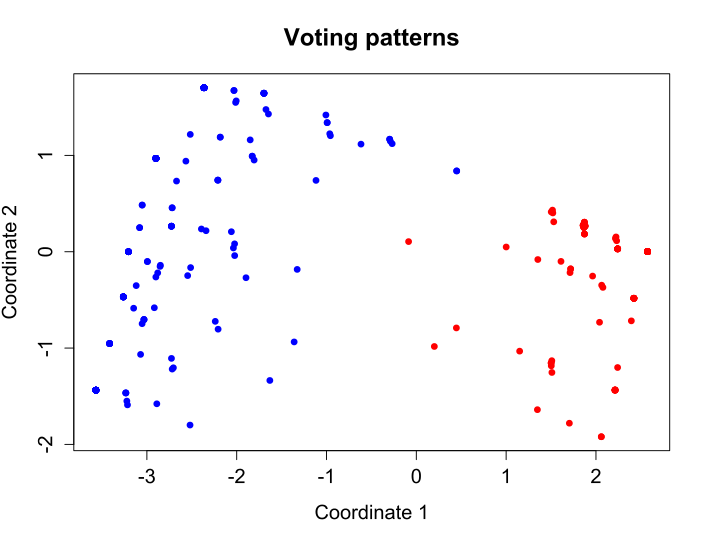
Classical Multidimensional Scaling of vote data from the United States House of Representatives. Each dot represents one Member of Congress and the color represents his or her political party (red for Republican, blue for Democrat). For each vote, a “Yea” was converted into a value of 1, a “Nay” into -1, and a “Present” vote equalled 0. The following ten votes were used for this image: H.R. 2642: Federal Agriculture Reform and Risk Management Act of 2013 H.R. 2609: Energy and Water Development and Related Agencies Appropriations Act H.R. 1564: Audit Integrity and Job Protection Act H.R. 1797: Pain-Capable Unborn Child Protection Act H.R. 3: Northern Route Approval Act H.R. 1911: Improving Postsecondary Education Data for Students Act H.R. 1256: Swap Jurisdiction Certainty Act H.R. 1960: National Defense Authorization Act for Fiscal Year 2014 H.R. 45: To repeal the Patient Protection and Affordable Care Act H.R. 1062: SEC Regulatory Accountability Act. [From the Wikipedia page on multidimensional scaling]

Data Set Characteristics:   Multivariate
Number of Instances:        435
Area:                       Social
Attribute Characteristics:  Categorical
Number of Attributes:       16
Date Donated:               1987-04-27
Associated Tasks:           Classification
Missing Values?             Yes
	
Origin:   Congressional Quarterly Almanac, 98th Congress, 2nd session 1984,
          Volume XL: Congressional Quarterly Inc. Washington, D.C., 1985.

Donor:  Jeff Schlimmer (Jeffrey.Schlimmer@a.gp.cs.cmu.edu)

Data Set Information:

This data set includes votes for each of the U.S. House of
Representatives Congressmen on the 16 key votes identified by the
CQA. The CQA lists nine different types of votes: voted for, paired
for, and announced for (these three simplified to yea), voted against,
paired against, and announced against (these three simplified to nay),
voted present, voted present to avoid conflict of interest, and did
not vote or otherwise make a position known (these three simplified to
an unknown disposition).

Attribute Information:

1. Class Name: 2 (democrat, republican)
2. handicapped-infants: 2 (y,n)
3. water-project-cost-sharing: 2 (y,n)
4. adoption-of-the-budget-resolution: 2 (y,n)
5. physician-fee-freeze: 2 (y,n)
6. el-salvador-aid: 2 (y,n)
7. religious-groups-in-schools: 2 (y,n)
8. anti-satellite-test-ban: 2 (y,n)
9. aid-to-nicaraguan-contras: 2 (y,n)
10. mx-missile: 2 (y,n)
11. immigration: 2 (y,n)
12. synfuels-corporation-cutback: 2 (y,n)
13. education-spending: 2 (y,n)
14. superfund-right-to-sue: 2 (y,n)
15. crime: 2 (y,n)
16. duty-free-exports: 2 (y,n)
17. export-administration-act-south-africa: 2 (y,n)


In R.

> install.packages("mlbench")
> data(HouseVotes84,package="mlbench")
> HouseVotes84
         Class   V1   V2   V3   V4   V5   V6   V7   V8   V9  V10  V11  V12  V13  V14  V15  V16
1   republican    n    y    n    y    y    y    n    n    n    y <NA>    y    y    y    n    y
2   republican    n    y    n    y    y    y    n    n    n    n    n    y    y    y    n <NA>
3     democrat <NA>    y    y <NA>    y    y    n    n    n    n    y    n    y    y    n    n
4     democrat    n    y    y    n <NA>    y    n    n    n    n    y    n    y    n    n    y
5     democrat    y    y    y    n    y    y    n    n    n    n    y <NA>    y    y    y    y
6     democrat    n    y    y    n    y    y    n    n    n    n    n    n    y    y    y    y
7     democrat    n    y    n    y    y    y    n    n    n    n    n    n <NA>    y    y    y
8   republican    n    y    n    y    y    y    n    n    n    n    n    n    y    y <NA>    y
9   republican    n    y    n    y    y    y    n    n    n    n    n    y    y    y    n    y
10    democrat    y    y    y    n    n    n    y    y    y    n    n    n    n    n <NA> <NA>
11  republican    n    y    n    y    y    n    n    n    n    n <NA> <NA>    y    y    n    n
12  republican    n    y    n    y    y    y    n    n    n    n    y <NA>    y    y <NA> <NA>
13    democrat    n    y    y    n    n    n    y    y    y    n    n    n    y    n <NA> <NA>
14    democrat    y    y    y    n    n    y    y    y <NA>    y    y <NA>    n    n    y <NA>
15  republican    n    y    n    y    y    y    n    n    n    n    n    y <NA> <NA>    n <NA>
16  republican    n    y    n    y    y    y    n    n    n    y    n    y    y <NA>    n <NA>
      .
      .
      .



Source: http://archive.ics.uci.edu/ml/datasets/Congressional+Voting+Records

Note: http://archive.ics.uci.edu/ml/datasets.html  is a wonderful dataset
repository.

The same techniques can be applied to bills in an effort to find bill clusters, or natural classes of bills that characterize voting blocks. Looking at this visualization sheds some light on what such pictures show.

Voting patterns for bills. Compare the actual vote break downs below and you will see that bills that clustered together do not necessarily receive uniform support from a party.

Party breakdown (yes votes):

Bill                         Republican Democrat
================================================
handicapped-infants          31         156
water-project-cost-sharing   75         120
budget-resolution            22         231
physician-fee-freeze         163        14
el-salvador-aid              157        55
religious-groups-in-schools  149        123
anti-satellite-test-ban      39         200
aid-to-contras               24         218
mx-missile                   19         188
immigration                  92         124
synfuels-corporation-cutback 21         129
education-spending           135        36
superfund-right-to-sue       136        73
crime                        158        90
duty-free-exports            14         160
export-act-south-africa      96         173

9.6.2. Basic ideas

We will begin by trying to motivate some of the basic ideas from an MDS perspective, because MDS emphasizes preserving similarity relations and understanding how LSI preserves similarity relations is key to understanding its utility in other applications.

The structure is as follows. First we pose the problem LSI solves as an MDS problem of a specific kind, and then discuss how LSI is an optimal solution. This in turn gives a good first approximation of the conditions under which LSI works best.

Footnotes

[1]

An important class of techniques for doing non-linear dimensionality reduction is called manifold learning. Manifold learning tries to generalize linear frameworks like PCA to be sensitive to non-linear structure in data. Usually manifold learning teachniques learn the high-dimensional structure of the data from the data itself, without the use of predetermined classifications of examples. Such learning algorithms are called unsupervised. Manifold learning techniques include isomap, locally linear emmbedding, spectral embedding, and multideminsional scaling.

[2]

This little exposition of LSI contains nothing that is not already said in Deerwester ([DEERWESTER1990]), Bartell et al. (1992), and Manning et al. (2003). The main purpose of this document is to bring the insights of all three together in one place. For an excellent discussion of the relation of LSI to factoring, see Tiago Ramalho’s blog