The study of the properties of social networks has been
an active area of research in sociology, anthropology, and social psychology for many decades,
as seen in some of the influential papers cited below, [MILGRAM1967], [GRANOVETTER1973] , [ZACHARY1977], and [FREEMAN1979],
and documented extensively in [WASSERMAN1994] and [NEWMAN2003A] . But due to some
seminal work in the 90s, coupled with
the explosion of the world wide web and the fresh interest generated
by social media, the field has entered a new phase of rapid growth.
It has also become clear that understanding
social networks involves understanding network properties
of relevance in a large number of disciplines.
One of the welcome consequences
is that there are large amounts of freely available data.
A good place to start is Jure Lekovec’s data page
known as the Stanford Large Network Dataset (SNAP) collection which has links to a great variety of networks, ranging
from Facebook style social networks to citation networks to
Twitter networks to open communities like Live Journal.
For smaller scale practice networks, try
Mark Newman’s data page.
Mark Newman is a physicist at the University of Michigan and Santa Fe Institute,
who has done a lot of important work on networks and written an excellent textbook;
The study of social networks is part of the larger discipline of the study
of systems, large entities with many interacting parts that
can function cooperatively (note the word can) to get things
done that none of the parts could get done alone. Systems include
The human body
Language (both computer and human)
Organizations such as the USSR, a boy scout troop, and
an automobile company.
The network of power lines across the U.S. and Canada
The internet
Political blogs on the Internet
The protein interactions in a living cell
A food web
Communities of people
But what about the network part? Why study systems as networks?
Systems that have parts that enter into recurring relations
may be pictured as networks. The system of the human
body has a subsystem called the central nervous system that
has parts called neurons connected to other neurons in complex
patterns; the way in which one neuron is linked to another,
however, is relatively uniform. Internet sites are linked to other
internet sites by hyperlinks; companies have hierarchical
structure in which the relation “is a superior of” recurs
over and over; power plants, power substation, and transformers
are linked together by high voltage transmission lines;
various functional units and organs of the human body are linked
together by various kinds of pathways
(circulatory, neural, and lymphatic). Species are linked to each other
by food dependencies ecologists call a food web.
The proteins in a living cell are linked to each other through
a network of interactions.
We may think of the parts as nodes
and the paths between them as links (or edges). This view of a system’s
functioning is the network view. Sometimes studying network
properties of a system, particularly a complex system that
passes through stages of growth, stability, and instability,
can reveal important things about how it works. Certain
nodes may be strategically placed so as to be vital to
normal function of the system. Certain substructures
may be recurring. Explaining some things about the network
requires knowing details about particular connections (local facts);
for example, in a food web, to explain a population decline
of some species in a food web, we might want to look at the predators
of that species. However, explaining functional properties
of the network may also require reference to global properties
(examples below).
Often our question about networks
involve local relationships, but the
answers lie somewhere in between the global and the very local.
For example, Yodzis (1998) compiled the results of a
number of experiments in which biologists removed a
predator from sequestered portions of ecosystems.
It certainly appears that the local effects would be quite predictable:
the size of the prey populations would increase.
But in fact, what Yodzis found was that the effects
were unpredictable. Some prey populations went up;
some went down. One of the complicating factors
is that a predator of species A might also
be a predator of some other predator of species A;
another is that some of the prey species may be competitors
for food further down the food chain. Thus an increase
in the population of prey Species A may entail a decrease
in the population of prey species B. It follows that policies
like killing seals in an attempt to bring back
the cod population (actually attempted in Canada in the late 1990s)
may actually harm the species they are intended to benefit.
The Figure below
shows David Levigne’s North Atlantic food web and gives a sense
of how staggeringly complicated food webs are. Decreasing
the number of seals would affect at least 150 other species.
For example, killing seals may have raised the populations of halibut
and sculpin, which also eat cod.
The moral of the story: Understanding the local effects of a small
change in highly interconnected networks often involves
looking at nonlocal effects.
There are really two very different kinds of goals
involved in studying networks, but
they lead us to very similar structural properties
of the networks. One is to find and exploit
structures that work efficiently for transmission
of effects through the network. This would be the goal of
a marketing analyst trying to find the best strategy
for spreading her message. Another is to understand
an existing structure to see what weaknesses and efficiencies it may have.
For example, the epidemiological study of a community of people
is concerned with what properties it has that promote
“efficient” transmission of a disease. Needless to
say, what is “bad” or “good” depends entirely on the purposes
at hand. What may be a bad feature from the epidemiolgist’s or
ecologist’s perspective
may be a good feature for the marketing analyst’s needs.
(For a demonstration of some basic ideas
motivating epidemiologists,
see Vax: a game about epidemic prevention.)
As we will see, the small world property that seems
to be a necessary feature for social networks entails
both kinds of efficiencies.
As the examples above
suggest, the study of networks plays a role in
a number of disciplines, and different disciplines
have developed different terminologies for
the same key ideas. The following
table summarizes some of the most important correspondences.
We will use the computer science term nodes and edges.
Thus a graph (or a network) is a set of
elements called nodes related in some regular way called
links, which we can picture in something like the following way.
Here, A, B, C, D, and E are nodes, and the lines
between them are edges. We define
a path in a network to be
a sequence of nodes connected by edges, and we will say
the above graph is connected,
because there is a path between any pair of nodes.
For example,
here are the four paths connecting A and D:
D E A
D E B A
D E C A
D E C B A
Path 4 includes all the nodes in the graph
and shows that graph is connected.
The length of a path is the number of edges
it traverses; the shortest path above, D E A, has length 2.
A number of important structural properties of graphs require
computing shortest paths or
the lengths of shortest paths.
There are many other sorts of information one might want to add
to graphs to keep track of properties of the
entities the nodes are modeling or of their relationships.
One of the most important ideas that the links between
the nodes may have strengths or weights that represent some
real world fact about how the entities are related.
For example, the network below is constructed
from some famous data about U.S. cities collected
by Donald Knuth. [KNUTH1993]
In this diagram of the Knuth data taken
from the networkx site,
the nodes are major cities, and the links between
cities are “weighted” by the distances between them.
Links are shown only for cities close to one another
(distances of more than 300 miles are ignored).
Rather than labeling the link “weights” with
numbers, the weights are represented by how
far apart the nodes on the graph are placed.
The graph clearly represents the clustering of
U.S. cities in the along coastlines, particularly
in the northeast.
In other graphs, link weight might represent
a variety of properties. For example, in the Enron
email network discussed in Section Visualizing Social Networks,
nodes are company employees and
a link between nodes represent the fact
that at least 5 emails have been exchanged between these
two employees. A weight on the link
might represent the volume of that email.
A key property of a node is how
many neighbors it has. This is called its degree.
In the example above, we see the following degrees:
Node
Degree
A
3
B
3
C
3
D
1
E
4
The degree distribution of a graph is a histogram
specifying for each possible degree how many nodes have
that degree. The highest degree in the above graph is 4.
1 node has degree 4, 3 nodes have degree 3, no nodes have degree 2, and 1 node
has degree 1. The degree distribution looks like this.
The reason to care about degree distributions
is that we can compare them with known
statistical distributions to learn things about the structural properties
of the graphs. It’s one of a number of global properties
of the graph that says something about how its
functioning can be orderly.
We turn next to one of the key tools in studying
the emergence of order in a complex system: Studying
random systems. In particular, we’ll look at random
graphs.
In a series of 8 ground-breaking papers published in 1959-1968,
Paul Erdos and Alfred Renyi (E&R) investigated
the properties of random graphs
and laid the foundations of
new area of graph theory. See for example [ERDOS1959] .
Random graph stage 1: The beginning, Netlogo simulation [WILENSKY2005].
Our chief interest in discussing some
of the properties of random graphs here is to
compare those properties with those of social networks.
Comparing orderly systems to random systems
gives us some insight into what properties
are key to the emergence of order.
The picture above (from
[WILENSKY1999] ) shows the generation of a random graph
by the following procedure, essentially due to E&R.
Choose a probability p for edge creation. The value of
p will determine how densely connected the graph is.
Start with a set of nodes (shown evenly distributed around the circle
in the first picture, although the layout
is not important) but with no connections between them.
Pick two nodes at random and add an edge between them with
probability p.
In the pictures above the graphs were redrawn after each
new link was added, using a force-spring layout algorithm,
which pulls linked nodes toward the center. In picture 2, small chain-like
components have formed. As time goes on, components
begin to merge, because an edge happens to be drawn between
two of their nodes, leading to picture 3.
In the last picture, picture 4, nearly all the nodes have been merged
into one giant component. (The
Netlogo model is here ).
[WILENSKY1999]
Since every link added increases the degree of two nodes,
the average degree of a node rises faster than the number of links.
A somewhat surprising result derived by E&R is that after the
average degree of a node exceeds one,
the growth of the giant component must accelerate very rapidly,
leading in very few steps to the creation
of a single giant component. This sudden global transformation
at very precise parameter value is called a phase transition
and the value of the parameter (average degree) is called a critical point.
Phase transitions are studied by physicists
concerned with phenomena like the transition
of a material from a liquid to a solid state
at its freezing point, or the transition
from a ferromagnetic state to a paramagnetic
state in a heated magnet, or superconductivity
emerging in certain materials at very low
temperatures. So random graphs play a key role
in the mathematics of critical phenomena,
which is called percolation theory.
The critical point for the emergence of a giant
component can be obsserved in the above simulation.
This corresponds in its statistical properties
to what physicists call a phase transition
(what happens at a certain temperature when water goes from liquid to
ice or when a magnetized piece of iron regains its magnetism).
This is one example of the strong conceptual connections
between the study of large networks
and statistical physics. [NEWMAN2004] cites a number of other examples.
A less surprising result that ER derived
has to do with the degree distribution of a random graph.
The degree distribution of a random graph is a
normal distribution, rather, the discrete counterpart
of a bell curve, a binomial distribution.
Here we see a normal degree distribution for a large random graph with 10000
nodes (not shown). The average degree of a node is 100 (so it’s fairly
densely connected), and as you can see, the frequencies peak at the average, and most nodes have edge counts right
around that average. This is characteristic of normal distributions,
a crucial feature of that famous bell-shape.
But the degree distributions of many real world
networks (such as the internet, many social networks,
and the power grid) look more like this.
This tells us that real world networks are not generated
by the kind of process that generates a random graph.
Another, perhaps unsurprising, result is that the average path
length in random graphs is quite low, typically
the log of the numbers of nodes. That means that
average path length grows much more slowly than the number of nodes.
This property is shared with social networks, as we
shall see, and is crucial in characterizing so-called
small world networks.
With this very brief sketch in place, we will try to
proceed by example, trying to illustrate a few of the important
research questions in social network study and how software
tools might play a role.
[ADAMIC2005] collected data from nearly 1500 political blogs
during the 2004 election, evenly balanced between conservative and liberal.
From this they constructed a network. They describe their
procedure as follows:
We constructed a citation network by identifying whether a URL present on the page of one blog references another political blog. We called a link found anywhere on a blog’s page, a “page link” to distinguish it from a “post citation”, a link to another blog that occurs strictly within a post.
An image of the network they found is shown below:
Political blog image. Layout via Fruchterman-Reingold algorithm. [FRUCHTERMAN1991]
Note the two great masses connected by a fragile bridge.
Same image with coloring of liberal and conservative sites
We start with a black and white image, laid out in a way that
tries to separate unconnected sites as much as possible,
resulting in two great masses connected by a bridge way of links.
The key point about the two masses is that the
graph layout algorithm uses no information about the liberal or conservative bias of the blogs. That
is, the two communities apparent in the uncolored diagram were
discovered by the layout algorithm because of the structure of
their mutual links. When we add the
coloring in the second figure, we see that the two communities
correspond very closely to the liberal and conservative blog
communities. The layout algorithm used is the
Fruchterman-Reingold algorithm, which is one of a family of
spring-directed algorithms. The idea of such algorithms is to
assume two competing forces, a repulsive force driving all nodes
apart and an attractive force keeping the nodes linked by edges
together. You can think of the edges as strong springs. Such
algorithms are good at discovering symmetries. For example, there is a
famous graph called the K-graph, which has 5 nodes, each symmetrically
to linked to the other 4. The figure below shows the K-graph
as computed by the default hierachical layout program in the popular
graphviz package, and as computed by Fruchterman-Reingold:
As can be seen, the hierachical layout algorithm does not succeed in
finding a way of both minimizing crossing lines and keeping all the lines
straight. Meanwhile, the force-directed algorithm moves nodes until the intrinsic
symmetry of the links brings the forces into equilibrium, at which point the nodes
lock into place. Another way to get an intuition for how a force layout
algorithm works is to see how it affects a graph as it grows.
Try out Ben Guo’s **Force Editor**.
Experiment with adding nodes, and especially with adding links between
existing nodes, and watch how the algorithm keeps finding symmetries
as new relationships are defined.
In the case of the blogs image, what holds the two community
masses together is a web of citation links; as Adamic and Glance
tell us
… 91% of the links originating within either the conservative or liberal communities stay within that community.
This result replicates that of other community studies
of liberal and conservative voices on the web,
such as that of [SUSSTEIN2001], which found that only
15% of liberal and conservative websites linked to
sites with opposing views; indeed, it replicates all
our experience of the politically polarized society
we live in, as represented in each day’s headlines.
Political pundits live in an echo chamber;
their world is structured so that they will hear only from those
saying the same things they are saying. Political
discourse may be the extreme case, but a number of studies have suggested
that this echo chamber effect
reflects a general property of communities.
The images above were made from
the original dataset, which is
available on
Mark Newman’s data page.
using Gephi[BASTIAN2009],
gephi.org, which is
an important graph visualization tool.
For more information about gephi and the specifics
of how this diagram was created, see Section Gephi.
Significantly, gephi is a Java program. Computing layouts for
large graphs (this one has 1500 nodes)
is a computationally intensive task.
Although layout algorithms often have termination
conditions (Fruchterman-Reingold has a concept
of an equilibrium state), as a practical matter
they are often not run to termination, but
until the information desired becomes apparent.
Thus, one needs to observe the evolution
of the graph and stop it at the appropriate point.
Moreover one may have to tweak a number of parameters
and try a number of different runs, each
for thousands of steps. In these
circumstances, efficient computation of
the step positions and efficient display
of the result is crucial, and Python may
not be the right tool
for the task. The python network module we
will introduce below, networkx, provides
an implementation of Fruchterman-Reingold,
and display facilities through matplotlib,
but the results are slow and not always pleasing to look
at.
The use of Gephi to produce the above picture
is a very clear case of the appropriateness principle
articulated in Section Why Python? .
Never use Python for the things it can’t do.
The [ADAMIC2005] paper presents some specific
evidence bearing on a very general problem. What
are the properties of a community? Are there
properties of network structure that can help
us find and define communities? In particular,
can we define community purely through the pattern of
connections among the members? The blog study
suggests the answer is yes, but the blog
example is both too easy and too hard, It
is too easy because these blog posts are unusually
focused on a single shared interest, politics; many sites
and many social relationships combine multiple
interests (sports, politics, religion, school ties).
It is too hard because the network
is too large to look at very closely. In the next section
we look at an example with a small group, and
find that community structure can still manifest
itself through strong interconnectedness.
10.1.6. Centrality and graph-partitioning: Zachary’s karate club
In 1977, anthropologist Wayne Zachary
published his study of a small karate club
[ZACHARY1977]. He represented the findings of his ethnographic
study as a graph, defined as follows:
A line is drawn between two points when the two individuals being represented consistently
interacted in contexts outside those of karate classes, workouts, and club meetings.
The diagrams below show
two views of the network he constructed, one using an algorithm
that simply positions the nodes on a circle,
the other using Fruchterman-Reingold (FR), are shown below.
Zachary’s karate club network: View 1 (Circular layout)
Zachary’s karate club network: View 2 (Fruchterman-Reingold layout)
Again, choosing the appropriate layout for a
graph proves to be revealing. What the
figure laid out by FR shows is that there are two key nodes, node
1 (actually the karate club instructor) and node 34,
(actually the club president), which are central to
different groups within the club. The next figure
uses the same layout and colors the two groups differently,
based on Zachary’s data. As can be seen, the two subgroups
Zachary found (which he called factions) correspond closely to the grouping the force-spring
algorithm finds, based on the interconnectedness of the nodes.
During the course of study, after a dispute between the
club president and the instructor,
the club split along the lines of the two factions shown above.
We would like to see whether it is possible
to define the two factions purely on the basis of structural properties
of the graph. The FR layout is one kind of evidence
that it is, but the two groups we find in the layout
are still largely matters of visual intuition. Note that
it is not clear how to derive two-colored graph from the
one-colored graph, because it is not clear exactly
where the boundaries of each group should be drawn, in
part because there are numerous inter-group
connections.
In this instance, one analytical concept that is clearly
important is graph centrality: Geometrically (or topologically,
as graph people sometimes say), this is the property
a node has when it is easily reached from all the other
nodes in the graph. Of course, graph centrality is not
necessarily represented by what is placed at the center of an image of the graph,
since different layout algorithms will place different nodes
(or no nodes at all) near the center. Thus graph centrality
first needs to be defined analytically, by making
precise exactly what relation that a node bears to other
nodes makes it central. And it turns out when this is attempted
that there are numerous different formal ways of defining centrality.
Two important concepts of centrality are
Degree centrality; and
Betweenness centrality.
We will provide some formulas and pointers for these concepts
in the appendix of this section; here we discuss the intuitions. The idea of degree centrality
is the simplest. The degree centrality of a node is just
its degree, that is, the number of neighbors it has. The more connected to other nodes
a node is, the higher its degree centrality. Thus, for example,
in the karate club graph, nodes 9 and 24 have degree centrality 5.
Degree centrality is clearly significant, but as can be seen
from the example, high degree centrality does not
correspond very well with cropping up often on paths between
other nodes in the network. This is better captured by
betweenness centrality [FREEMAN1979].
Betweenness centrality has to do with how often a node crops up
when taking a best path (there may be
more than one) between two other nodes. The
betweenness centrality of node n is
defined as the proportion of best paths between any other
pairs of nodes which pass through n. By definition
the betweenness
centrality of n
depends on the connection properties of every pair of nodes in the graph,
except pairs with n, whereas degree centrality depends
only on n’s neighbors. A very closely related notion
is the notion of betweenness for edges. Given
the set of shortest paths between all node pairs,
the edge centrality of e is simply the proportion
of those which pass through e. To get a
better feel for the intuition, it often helps to think
of a network as having traffic: Travelers start out
from each node with their destinations evenly divided
among the other nodes, always choosing best paths for
their journeys. In this situation, the node with the highest
betweenness will have the most traffic.
Interestingly, in the case of the karate club, degree centrality
and betweennness centrality give similar results:
Nodes 1 and 34 are the top-ranking nodes by both measures,
in accord with our intuitions of their centrality.
When you think carefully about the case of social networks,
the problem of centrality becomes much more interesting
and much more difficult. What do we mean when we speak
of social centrality? What do we have in mind when we speak
of it as a social network concept? One thing that
comes to mind is social status or importance (as
in Very Important Person), but it is not at all
clear that social status can always be deduced from
the kind of social networks we have been looking
at, or that it directly maps onto what we think
of as centrality. The two most central nodes in Zachary’s karate
network probably do have high social status, but that’s not what
makes them interesting. What makes them interesting is
that they perform some sort of key role in maintaining
social cohesion. So network centrality is a kind of
role a node has in the graph, deduceable from the link
relations, and its exact meaning will depend
on the exact definitions of the links. In
many social networks, a link between two nodes just means
“know each other”. In Zachary’s
graph, the kind of relation pictured by a link is
“a friendship”, which is a social tie closer
than acquaintance (since all the club members
are acquainted); and it’s that fact about Zachary’s graph
that gives centrality the particular meaning it has (“being
at the center of a network of friends”).
The following graph is a famous graph of the relationships
by marriage of 15th century Florentine Families.
Here betweenness centrality does a pretty decent job capturing
our historical (and visual!) intuitions.
Family
BC
Medici
.522
Guadagni
.255
Strozzi
.103
So the relationship
of relation by marriage does capture something socially significant
about family relations, directly enough so that betweenness
centrality correctly captures a notion of social centrality.
But what these examples also suggest is that there may not be
one definition of centrality suitable for all
social networks. The exact definition
will depend not just on the network
but also on our social science goals. [NEWMAN2003]
considers the example of a sexual contact network,
where the primary goal is to make predictions
about the probable transmission paths
of sexually transmitted diseases. The relevance
of the concept of betweenness is clear, but
Newman argues that betweenness centrality (B.C.) as defined
above is not the right kind of centrality. To find all the nodes
of importance in the network, we don’t want
a computation that just considers shortest
paths. A virus traveling through such a network
will not necessarily take the shortest path;
it will essentially take a random walk.
Thus, what we want for our betweenness measure of a node
is to compute what proportion
of random walks starting and ending at all possible
node pairs pass through .
Newman defines such a concept of random-walk betweenness
and then shows that although it has a high correlation with B.C.,
it can value nodes left out by B.C. because
they lie on few shortest paths. (See the figure below, from
[NEWMAN2003], which has arrows pointing to several such nodes for a sexual
contact network).
Centrality measures can tell us what nodes might be at the centers of
communities, but they don’t directly tell us what those communities are.
What we need beyond that is an analytical method for splitting a network
into communities (a divisive algorithm) —
or conversely, a method for collecting individual
nodes into larger and larger communities
(an agglomerative algorithm).
There are actually many graph-partition (or community discovery)
currently in the literature, many available in Python implementations.
The most complete collection of such algorithms is in igraph,
a competitor of networkx originally developed in R and ported
to Python. One of the most popular algorithms
is the so-called Louvain algorithm [BLONDEL2008],
which seeks a partition of the graph that maximizes a
quantity called modularity. Louvain exists in igraph
under the name community. There is also a Python
version for networkx available in
the module python-louvain.
Here, we will sketch another algorithm
as an example, choosing an elegant divisive algorithm
known as the Girvan-Newman algorithm[GIRVANNEWMAN2003],
because it is conceptually one of the simplst community
discovery algorithms. It
depends on computing edge-betweenness values. Begin by considering
the graph below.
B’s links to D and C are different from B’s links to A, E and F.
A, E, and F are part of a tight knit community where the people
largely all know each other, and B is part of that community too.
But B doesnt know any of the people C or D know. The links
between B and C and B and D are community-spanning. The links
between B and E, A, and F are within-group.
Note that removing the links from B to C and D
splits the network into its 3 tightly knit subcommunities.
Thus, one approach to community discovery is to remove the
community-spanning edges until the graph splits into
unconnected components. Those components will
by definition be communities. In this case, removing (B, C)
gives us 2 components, and then removing (B, D) gives us three.
But how do we find “community-spanning edges” (more commonly called
local bridges)? It turns out that the concept of
edge-betweenness, introduced above in discussing centrality, does a
very good job finding local bridges.
Edge betweenness is a measure of what proportion
of all shortest paths an edge lies on. In the graph above,
the node labeled D only lies
on the shortest paths of edges in its own community (7 and 8). B on
the other hand, lies on the shortest paths between all the edges in
D’s community (6,7,8, and D) and all the edges in A’s community
(A,1,2,E,F), adding up to 20 pairs. Thus the edge (B,D), which
connects B to the D community, will have high betweenness. But B also
lies on all the shortest paths between the D-community and the
C-community, so (B,D) gets still more betweeness points in virtue of
falling on the shortest paths between all the D-community edges and
all the C-community edges (another 16 shortest paths). For similar
reasons the (B,C) edge will be high scoring, because it lies on the
best paths between the D-community and the C-community, and between
the C-community and the A community.
The following sketch of the Girvan-Newman method is a very slightly modified
version of the sketch given in [EASLEY2013] (p. 76). The
method relies on the idea that edges of high edge-betweenness
tend to be community-spanning.
Find the edge of highest betweenness — or multiple edges of highest betweenness,
if there is a tie — and remove these edges from the graph.
This may cause the graph to separate into multiple components.
If so, these are the largest communities in the partitioning of the graph.
With these crucial edges missing, the betweenness levels of all
edges may have changed, so recalculate all betweennesses, and again
remove the edge or edges of highest betweenness. This may break some
of the existing components into smaller components; if so, these are communities
nested within the larger communities found thus far.
Proceed in this way as long as edges remain in graph, in each step recalculating
all betweennesses and removing the edge or edges of highest betweenness.
This very elegant algorithm thus finds the very largest communities
first, and then successively smaller communities nested within
those. As simple as it is to describe in words, it is
quite computationally costly because each step requires finding
the best path between all pairs of remaining nodes.
Returning to the example of the Karate club, the first edge removed
is the (1, 32) edge. Recall that our two highest betweenness nodes
were 1 and 34. Not surprisingly, (1,32) lies on the shortest path
between them. However, removing the (1,32) edge does not divide this
densely connected graph in 2. We continue removing edges as in step 2
until the graph is broken into two
components and we have:
This corresponds very closely to Zachary’s data-driven split,
but not exactly. Edges 3 and 9, the boundary edges that seem to
participate in the most connections between both groups
have been placed in the group centered round 34 instead
of the group centered round 1. For a discussion
of a Python implementation of this algorithm, as well
as the analytical network measures discussed in this
section, as well as some additional measures see Section Introduction to Networkx.
The notion of local bridge, or community-spanning edge, or high
betweenness edge, corresponds very closely to an important concept in
sociology known as a weak tie, introduced in a much-cited 1973
paper by Mark Granovetter entitled “The strength of weak ties”
[GRANOVETTER1973] . Setting out to study how people got jobs in the
(then) working class community of Newton, Massachusetts, Granovetter
asked each of the workers in his sample “How did you get your current
job? Was it through a friend?” The recurring answer was “No, it was
an acquaintance.”
Granovetter’s explanation appealed to a property of social networks:
The overall social structural picture suggested by this argument can
be seen by considering the situation of some arbitrarily selected
individual-call him Ego. Ego will have a collection of close friends,
most of whom are in touch with one another – a densely knit clump of social structure.
Moreover, Ego will have a collection
of acquaintances, few of which know each other. Each of
these acquaintances, however, is likely to have close friends in his
own right and therefore to be enmeshed in a closely knit clump of
social structure, but one different from Ego’s. [GRANOVETTER1983] .
The point is that members of Ego’s own densely knit group are less
likely to know something Ego doesn’t know, or to have contacts Ego
doesn’t already have. When it comes to job hunting, new information
and new contacts are key. On the other hand, weak ties by definition
are connected to other tightly knit groups with new information and
new contacts, and some of those weak ties
are what Granovetter calls bridging weak ties,
which lead from one community to another, creating an even greater possibility
of novelty. So in the context of a job search, weak ties will be of
much greater importance. More generally, weak ties will take on
greater importance in any context where a change of social status or
social practice is at issue:
Getting a job
Starting a new business
Finding a mate
Learning new information
Spreading a social innovation, such as a new kind
of technology, or a political movement.
The converse of this observation is that the absence
of weak ties can be devastating, leading to community
isolation and poor access to resources.
Along with the idea of the stength of weak ties goes
a particular picture what social networks look like.
They look, roughly, like the graph above, islands
of tightly knit groups connected by local bridges.
This conception provides a concrete social
context for the later concept of a small world.
In 1967, Stanley Milgram of Harvard University conducted the following
experiment. He asked 300 people chosen at random
to send a letter through friends to a stockbroker near Boston we will call the
target. If they had never met the target, they were asked
to pass the letter, along with the instructions, on to a friend whom they felt might
be “closer to” the target.
There was some uncertainty about how well this experiment design would work.
Would letters simply be cast aside when the target was unknown?
If they were forwarded, would they be forwarded to recipients
who actually could get the letter closer to the target?
The results were astonishing: 64 of the original 300 letters arrived
safely. The average length of
the recipient chain for those 64 letters was 5.5 persons.
What Milgram had shown was that on average, the chain of
acquaintances linking any two people is 6 people long. (The
experiment has been successfully replicated many times).
Playwright John Guare coined the term six degrees of separation
for this new conception of how linked together we all are in
the modern world.
What Milgram’s experiment shows is that social networks
are small worlds. The term is being used informally
here, as in “It turns out my sister-in-law’s cousin is
married to my dissertation advisor. Small world!”
As we shall see shortly, the term can be given a
precise definition.
Some years after Milgram’s initial study the idea of a small world
resurfaced multiple times in a series of studies of networks by
a diverse set of researchers [BARABASI2002], covering
topics as diverse as the world wide web, citation
networks among physicists, neural nets, and the power
grid of the Western United States. It
became apparent that small world networks were
important in a number of different disciplines. In
fact, it began to seem as if most of the networks
of interest in the real world were small world networks.
To get to this point, it was first necessary
to get clear on what small world networks were.
This was the key contribution
of Duncan Watts and Steven Strogatz [WATTS1998] . Watts and Strogatz begin with the observation
that many real world networks lie between the extremes
of random connection and connection by some regular
pattern (such as models of crystal structure). Thus
they propose to explore a set of networks that can
be constructed by beginning with a regularly
connected network and adding random rewirings.
This netlogo model,
illustrates the
idea. The nodes are arranged in a circle, with each connected to
the neighbor on either side. In the diagram below, each
node begins being connected to 4 of its neighbots.
One step in the network generation process
is completed by doing the following (acheived in the Netlogo
simulation by pressing the rewire one button):
Visit an edge. Rewire it with probability p, detaching one of its connections
at one end and reattaching it to a randomly chosen node somewhere in the circle.
A network is generated by repeating this step for all the nodes in the network.
The higher the probability of rewiring p, the more randomness is introduced
into the network. (In the Netllogo simulation,
the entire sequence of steps can be run through rapidly
by pressing the Rewire all button.)
The first graph is totally regular. The probability of
rewiring is 0. The third graph is totally random. All
the initial regular links have been rewired to random places.
The middle graph is somewhere in between, and this is where
we find what W&S call small worlds..
To describe the range of network structures
from ordered to random, W&S make key use of two global properties of
network structure:
Average Path Length (APL): Average path length is calculated by finding the shortest path
between all pairs of nodes, adding them up, and then dividing by the total number of pairs.
This shows us, on average, the number of steps it takes to get from one member of the
network to another. In the totally ordered graph, APL is quite high.
There are no short cuts for getting from one side of the graph to
the other. The random graph lowers APL dramatically, because
each random rewiring generates dramatically reduced shortest paths
for a number of nodes.
Clustering Coefficient (CC):
The clustering coefficient of a node is the ratio of the number of links connecting a node’s
neighbors to each other to the maximum possible number of such links. The clustering
coefficient of a graph is the average clustering coefficient of all the nodes
in the graph. In the ordered graph, clustering is quite high; the neighbors
a node n is connected to are quite likly to be connected to other
nodes n is connected to. In a random graph, the clustering coefficient is
dramatically reduced, because those predictable links have all been destroyed.
Watts and Strogatz define what they call small worlds as follows:
Small world
A network with a low APL and a high CC
is called a small world. [1]
Let’s consult our intuitions about social networks
and guess how these two quantities should look in human social networks.
The clustering coefficient (CC)
measures the “all-my-friends-know-each-other” property (sometimes
summarized as the friends of my friends are my friends). The higher
the clustering coefficient of a person the greater the proportion of
his friends who all know each other. Thus, our intuitions suggest that
social graphs will have high CCs.
This property
is utterly unlike random graphs.
By the same token, it seems,
human social networks should have high APLs.
If our friends more or less know all the same
people we do, then the world is
just a collection of cliques, and
paths from one clique to another will
be hard to come by. Thus, APLs should be high. In fact, our intuitions
are right about CCs, but
Milgram’s experiment shows that they are completely
wrong about APL: Human social networks
actually have low APLs, and this is
like random graphs. Summing it up:
Thus, human social networks are small worlds.
With this simple definition, W&S succeeded not only in
isolating some key properties of social graphs, but in
identifying key structural properties
that characterized a large class of real world networks of great interest.
The figures above illustrates the basic idea. For
p=0, we get total regularity, which
is characterized by a high APL and a high CC;
for p=1, we have
a random graph, with both low CC
and low APL. The middle graph
was constructed with * p* =.1, and at that value
we get what W&S call a small world, still a high CC,
because few of the original
regular groups have been broken up, but with
an APL almost as low as that of the random graph. The
chief surprise is just how
quickly a few random connections lower the APL,
effectively transforming a network into a
collective through which information can be efficiently spread.
A little chaos is a good thing.
W&S demonstrate the applicability of
their definition of social networks
with three very different examples:
Collaboration network of Hollywood actors
The power grid of the Western United States
The neural network of the worm Caenorhabditis elegans[2]
Each of these has a small world graph
and each is a proxy for an
important class of networks.
The C. elegans connectome, which consists of 302 neurons
hardwired into one permanent configuration. (From Stanford CS379c site)
Thus, the actor collaboration
graph is of course a proxy for any social network, the C. elegans graph
is a proxy for any network of neurons, including the human
brain, and the power grid a proxy for any
physical network transmitting resources (including information).
We will shortly add a very important additional
physical network, the Internet, to the list of
small world graphs.
Crucially, W&S also show the APL/CC properties have functional consequences
for how information or resources spread through the graph.
They apply a simple model of disease spread and show
that infectious diseases will spread much more easily
and rapidly in a small world than in a randomly connected graph.
Note that it is precisely the combination of low
APL and high CC that provides the ideal conditions
for a worldwide pandemic like the Influenza pandemic of 1918,
which traveled along all major trade routes
(and was also aided by swarms of
returning soldiers, dispersing through their homelands).
Small worlds arise in graphs that maintain a tension
between two kinds of graph properties, communities that are tightly
knit and efficient connectedness of the entire graph.
This is exactly Granovetter’s picture of a social network, tightly knit communities
linked by weak ties. Each time we rewire a link
in the W&S simulation, we are adding a weak tie to the network
(and reducing the APL by a significant amount). The functional consequence of
adding those weak ties, that information can efficiently
reach a large proportion of the nodes in the graph, is
exactly what Granovetter getting at in the title
of his paper, “The Strength of Weak Ties.”
As the influenza example shows, this strength can also be a weakness.
What makes the study of networks as networks fruitful
is that the same structural properties can enable multiple
functions.
Suppose we start with a network with two connected nodes and then begin
adding nodes; each time we add a node we decide whether
to attach it to other nodes using the following simple
rule: the more “popular” a node the more likely
it is to be connected to by new nodes. Mathematically it looks
like this:
That is the probability of an existing node being chosen
for a connection () is proportional
to its degree , and is equal
to the proportion of all the links in the network
that connect to .
This strategy is
called preferential attachment.
Networks created by this procedure,
originally proposed in Barabási and Albert [BARABASI1999] ,
are also referred to as Barabási-Albert
networks. The procedure differs in two important
ways from the one we described for generating random graphs.
The graph grows during the generation process,
which means that older nodes have a better chance
of having high degree, and nodes with more links
are preferred when attaching.
Both these differences contribute to making
graphs that correspond better to properties of
certain real world networks.
An example is shown below.
A Barabasi scale-free network in the making (the picture
is a snapshot of a simulation created using NetLogo). This network has 227
nodes. Note how hubs have become to emerge (high-degree
nodes placed at the center of a cluster). That is, there
is a very clear minority of nodes that spawn a much higher than
average number of connections.
The kind of degree distribution
that results from this procedure
is shown in the following plots.
This kind of distribution is called a scale-free or power law
distribution.
The name power law comes from the fact that the probability
of having a particular degree k degree
is proportional to k raised to a negative exponent :
Typically, in power law distributions, .
It turns out that if we remove
either growth or preferential attachment from
the Barabási-Albert procedure, we no
longer get a power law distribution.
In a power-law distribution,
the probability of an
outlier at a particular degree is a small, but
the summed probabilities of the outliers is quite large.
As a result, some outliers of high degree (hubs) are to be expected.
The graphs below, generated from the above Netlogo
simulation, illustrate this. The top plot is a histogram of node degrees.
The number of nodes exhbiting a particular
degree falls very rapidly as the degree rises, but what this
means is that there is a small but very important set of nodes with
very high degrees (hubs). If we map this on a log scale (the
bottom diagram), we see that the number of nodes of
a particular degree decreases at an approximately
linear rate: Power law histograms look linear
on a log scale.
Roughly what is going on is this:
if there is 1 node with a degree of 1000,
then there will be 10 nodes with a degree
of 100, and 1000 nodes with a a degree of 1.
Unlike normal distributions, power law distributions do not have a peak at the average, and they
are much more likely to contain extreme values.
Because the summed counts of
the rarer events at the right (nodes of very high degree)
are quite high,
hubs with very high degrees are virtually guaranteed.
This property
gives the distribution what is often referred to as a long tail
or a heavy tail. A lot of the probability mass
is to be found on the right, in the tail of the curve:
There are a lot of very rare events
that are more or less equally likely to occur (the probabilities
of hubs with degree above 100 or hubs with degree above 1000 are not that
different), so this can make actual samples look
quite noisy at the tail (as can be seen in the
histograms made from the Netlogo simulation).
So the contrast with the normal distributions
we found in random graphs is quite clear.
With normal distributions, extreme outliers are
extremely unlikely. With power law distributions,
they are virtually certain.
The lesson of the Barabasi-Albert work
is that when we look at real world networks, we find
outliers everywhere.
Consider two examples discussed by Barabasi and Albert
[BARABASI2002].
The actor’s collaboration network of Duncan and Watts.
41% of the actors have fewer than 10 links. This statistic
follows from a fact known to all actors. Most actors
are not very well known and appear in very few movies.
In addition, however, there are hubs, actors with an astounding number
of links. John Carradine has 4000 links. Robert Mitchum
has 2905. Such extreme outliers have vanishingly
small probabilities in a random model, but are to be expected
in a power law model. The hubs are the key structural element
responsible for the small world effect. Remove these hubs from
the network and the average path length climbs.
The internet. Some sites are just hubs. The latest web survey
cited by Barabasi [BARABASI1999], covering
less than a fifth of the web, found 400 pages with 500 incoming
links and one document with over 2 million incoming links.
The chance of any one of these occurring in a random graph
the size of the web is less than . The change of 500 such
nodes is virtually 0.
The interesting thing is that Barabasi-Albert graphs
are also small worlds. They have a high clustering
coefficient and, thanks to hubs that connect different
neighborhood, they also have low average path lengths.
But because the process that produced them
creates hubs, they model the degree distribution
of many real world networks much better than
Watts-Strogatz graphs. The degree distributions
of Watts-Strogatz graphs looks like that of a random graph:
node degrees all cluster around the average and
the probability of outliers is vanishingly small.
The reason for this is the Watts-Strogatz generation
process: The
rewirings that lower the average path length in the Watts-Strogatz
model are random.
On the other hand,
the processes that build real world networks are
definitely not. Acting roles in movies are not handed out
by independent coin flips.
Actors who have appeared in many movies are far more likely
to get new roles than actors who have appeared in only one movie.
Web pages that have been linked to 499 times are far more likely to be noticed
and attract a 500th link than obscure pages that have been linked to
only once. In general, there is a large
class of networks in which nodes with lots of connections are more likely
to get further connections, a pattern that has been
called the “rich-get-richer” principle.[#fn3]_
The mechanism of preferential attachment directly models that
principle.
This does not mean that all real world small worlds
are power law graphs; for example, the neural
network C. elegans is not. It is structured
by different organizing principles. Yet a very important
class of real world networks are power law networks. [4]
Morevover, the importance of power law distributions extends far beyond
network degree distribution. [NEWMAN2005] discusses a number
of examples, which include both network and non network cases.
These include two examples well-known among social
scientists, Zipf’s law, and Pareto’s Law.
Numbers of occurrences of words in the novel Moby Dick by Herman Melville.
(The frequency distribution of words is a well studied example of
a power law distribution, observable in all kinds of texts in all
languages. It is often called Zipf’s Law because of
the work of George Zipf, who studied it extensively [ZIPF1949].)
Numbers of citations to scientific papers published in 1981, from time of
publication until June 1997. (network)
Numbers of hits on web sites by 60000 users of the America Online
Internet service for the day of 1 December 1997.
Numbers of copies of bestselling books sold in the US between 1895 and 1965.
Number of calls received by AT&T telephone customers in the US for a
single day. (network)
Magnitude of earthquakes in California between January 1910 and May 1992.
Magnitude is proportional to the logarithm of the maximum amplitude of
the earthquake, and hence the distribution obeys a power law even though
the horizontal axis is linear.
Diameter of craters on the moon. Vertical axis is measured per square
kilometre.
Peak gamma-ray intensity of solar flares in counts per second,
measured from Earth orbit between February 1980 and November 1989.
Intensity of wars from 1816 to 1980, measured as battle deaths per
10000 of the population of the participating countries.
Aggregate net worth in dollars of the richest individuals in the US in
October 2003. (This kind of distribution of wealth example is one of
the oldest known power law distributions, first observed by
Pareto [PARETO1896].) Pareto’s law says that 80% of the wealth is
held by about 20% of the people. [NEWMAN2005] shows this relationship
obtains when the exponent ( above) is about -2.1.
Frequency of occurrence of family names in the US in the year 1990.
Thus, while many real
world phenomena follow normal distributions
with peaks at the average (for example, the heights of males,
or the speed of cars), a significant set of phenomena
do not. Of course, knowing that some real phenomenon
follows a power-law distribution does not
tell us what particular mechanism is responsible for the distribution. The next step
is to to find a plausible mechanism. In some cases,
the elements of the distribution are in a network
with both the key features of the Barabasi-Albert
procedure: (a) some kind of growth process is responsible
for the emergence of the extreme examples; and (b)
some kind of rich-get-richer principle
governs the growth process. This seems
to be the right view of internet websites and
the actor network. But this kind of explanation
does not seem to play a role in crater size, wealth
distribution, or forest fire sizes. [NEWMAN2005] and [NEWMAN2010] reviews
a number of other possible mechanisms that have been
proposed. Of particular importance is the
concept of self-organized criticality, used, for example, in [DROSSEL1992]
to derive a power law distribution for wild fire areas.
The utility of graph layout algorithms in discovering community structure.
The importance of centrality measures in discovering influential
or important nodes in a network.
The utility of graph partition algorithms like Girvan-Newman in defining
communities within a graph. This in turn relied heavily on the notion
of edge-centrality.
Random graphs are important in the study of networks, acting as a kind
of background against which the structure of various kinds of graphs
can be compared.
Weak ties are important aspects of social structure, especially
where the diffusion of information or resources is concerned.
Small worlds correctly model certain key aspects of social structure,
specifically the way social networks are organized into tightly
knit cliques connected by weak ties. The result is high clustering coefficient
and low average path length.
Power law networks capture key aspects of many real world networks which are not captured
by the small world model. Barabasi-Albert power law networks have a power law or scale-free degree distribution and they are small worlds.
Examples include social networks such as the actor collaboration network and the world wide web.
[BUCHANAN2002] Summarizes key developments in the emerging
field of network science, and does an excellent job drawing
the connections (no pun intended) and explaining the
significance. Short-listed for the Aventis Science Writing Prize in 2003.
[BARABASI1999] Summarizes much of the important work
of the 90s, like Buchanan, but more focused
on power-law properties of networks and related issues.
[EASLEY2013] General very readable textbook bringing together
a lot of different aspects of network studies.
[CHRISTAKIS2009] Focused more on the real world properties
of social networks. The social science side of the picture.
[WATTS2003] Small world model, its development and consequences,
including some fascinating stuff on epidemiology.
In this appendix, we give some formulae for the measures introduced above.
First we introduce some conventions for sets and statistics
we want to collect for a node :
Note that is not in the neighborhood set .
Then the clustering coefficient for node , written , is defined as
As stated above
is the maximum possible number of edges connecting neighbors of (the number
of edges there would be if all of ’s friends knew each other),
so is the number of actual edges between
neighbors of divided by the maximum possible number of
edges between neighbors of . The clustering
coefficient of a graph is just the average of this number for all
nodes in a graph.
As an example, consider the graph
This is the graph we used in What are networks?.
What is the clustering coefficient of E in this graph?
E has 4 neighbors, which means there are 6 pairs among them.
Of those 6 pairs, none of the 3 pairs with D are
linked, since D is linked only to E. THe other 3 all
know each other, (A,B), (A,C), and (B,C). This
means , the clustering coefficient
of E, is computed as follows:
For the average path length in this graph consider that we have
5 nodes, which means there are
Of these 10, all the shortest paths are of length 1 except for 3 paths
involving D: (D,C), (D,A), and (D,B) are all of length 2, so
we have:
We define the betweenness centrality of node , written as
Here is the total number of shortest paths
from to and is the total
number of such paths which pass through . The symbol indicates
we sum that quantity for various and , and
the little subscript tells us ; that is, we find that quantity
for all nodes in the graph that are distinct from .
As another example, consider the graph
We will compute the betweenness of the nodes D and E. The betweenness of D is 0, because
D does not lie on the shortest path for any pair of nodes, so
is always 0. The betweenness of E is more interesting. E lies on shortest paths
between the following
pairs: A and B, A and D, B and D, C and D. The shortest paths
between A and D and between B and D are unique, but there are multiple shortest paths
between C and D and between A and B.
Both of the shortest (C,D) paths pass through E,
but only one of the shortest (A,B) paths passes through E.
So the betweenness computation looks like
this:
Questions
How does the betweenness computation for node E change if we add an edge
between C and E as follows?
How does the betweenness computation for node E change if instead we add an edge
between A and B?
Betweenness centrality is often normalized to give a score between 0 and 1.
To see thow this works, note that each of the terms in the betweenness sum is a number
between 0 and 1. We just take their average. All the examples above involve the same
number of nodes, therefore the same number of pairs, so in all cases we divide by
6. For the first example, 3.5/6 is .583. The general expression for
the number of possible pairs of k things is given in the table above:
If we have a graph of nodes, the betweenness computation for any
one of them will involve other nodes, so the number of
possible pairs of things is
For example, the graph above has 5 nodes, so in computing the betweeneness
of any node , we have pairings
of other nodes. The normalized betweenness divides the
betweenness by that number to get the average betweenness score
for paths through .
Compute the normalized betweenness for the graph in Question 2.
What is the degree centrality of node E in the graph in Question 2?
What is the clustering coefficient for node E in the graph in Question 2?
What is the average path length in the graph in Question 2?
10.1. Social Networks
The study of the properties of social networks has been an active area of research in sociology, anthropology, and social psychology for many decades, as seen in some of the influential papers cited below, [MILGRAM1967], [GRANOVETTER1973] , [ZACHARY1977], and [FREEMAN1979], and documented extensively in [WASSERMAN1994] and [NEWMAN2003A] . But due to some seminal work in the 90s, coupled with the explosion of the world wide web and the fresh interest generated by social media, the field has entered a new phase of rapid growth. It has also become clear that understanding social networks involves understanding network properties of relevance in a large number of disciplines. One of the welcome consequences is that there are large amounts of freely available data.
A good place to start is Jure Lekovec’s data page known as the Stanford Large Network Dataset (SNAP) collection which has links to a great variety of networks, ranging from Facebook style social networks to citation networks to Twitter networks to open communities like Live Journal.
For smaller scale practice networks, try Mark Newman’s data page. Mark Newman is a physicist at the University of Michigan and Santa Fe Institute, who has done a lot of important work on networks and written an excellent textbook;
CMU CASOS data sets.
NCEAS Interaction (Food web) data sets.
UCINET Datasets.
Vladimir Batagelj and Andrej Mrvar’s Pajek Datasets.
Linkgroup’s list of datasets.
Barabasi lab datasets.
Alex Arenas’s datasets
10.1.1. Why study networks?
The study of social networks is part of the larger discipline of the study of systems, large entities with many interacting parts that can function cooperatively (note the word can) to get things done that none of the parts could get done alone. Systems include
The human body
Language (both computer and human)
Organizations such as the USSR, a boy scout troop, and an automobile company.
The network of power lines across the U.S. and Canada
The internet
Political blogs on the Internet
The protein interactions in a living cell
A food web
Communities of people
But what about the network part? Why study systems as networks? Systems that have parts that enter into recurring relations may be pictured as networks. The system of the human body has a subsystem called the central nervous system that has parts called neurons connected to other neurons in complex patterns; the way in which one neuron is linked to another, however, is relatively uniform. Internet sites are linked to other internet sites by hyperlinks; companies have hierarchical structure in which the relation “is a superior of” recurs over and over; power plants, power substation, and transformers are linked together by high voltage transmission lines; various functional units and organs of the human body are linked together by various kinds of pathways (circulatory, neural, and lymphatic). Species are linked to each other by food dependencies ecologists call a food web. The proteins in a living cell are linked to each other through a network of interactions.
We may think of the parts as nodes and the paths between them as links (or edges). This view of a system’s functioning is the network view. Sometimes studying network properties of a system, particularly a complex system that passes through stages of growth, stability, and instability, can reveal important things about how it works. Certain nodes may be strategically placed so as to be vital to normal function of the system. Certain substructures may be recurring. Explaining some things about the network requires knowing details about particular connections (local facts); for example, in a food web, to explain a population decline of some species in a food web, we might want to look at the predators of that species. However, explaining functional properties of the network may also require reference to global properties (examples below).
Often our question about networks involve local relationships, but the answers lie somewhere in between the global and the very local. For example, Yodzis (1998) compiled the results of a number of experiments in which biologists removed a predator from sequestered portions of ecosystems. It certainly appears that the local effects would be quite predictable: the size of the prey populations would increase. But in fact, what Yodzis found was that the effects were unpredictable. Some prey populations went up; some went down. One of the complicating factors is that a predator of species A might also be a predator of some other predator of species A; another is that some of the prey species may be competitors for food further down the food chain. Thus an increase in the population of prey Species A may entail a decrease in the population of prey species B. It follows that policies like killing seals in an attempt to bring back the cod population (actually attempted in Canada in the late 1990s) may actually harm the species they are intended to benefit. The Figure below shows David Levigne’s North Atlantic food web and gives a sense of how staggeringly complicated food webs are. Decreasing the number of seals would affect at least 150 other species. For example, killing seals may have raised the populations of halibut and sculpin, which also eat cod. The moral of the story: Understanding the local effects of a small change in highly interconnected networks often involves looking at nonlocal effects.
David Levigne’s North Atlantic food web
There are really two very different kinds of goals involved in studying networks, but they lead us to very similar structural properties of the networks. One is to find and exploit structures that work efficiently for transmission of effects through the network. This would be the goal of a marketing analyst trying to find the best strategy for spreading her message. Another is to understand an existing structure to see what weaknesses and efficiencies it may have. For example, the epidemiological study of a community of people is concerned with what properties it has that promote “efficient” transmission of a disease. Needless to say, what is “bad” or “good” depends entirely on the purposes at hand. What may be a bad feature from the epidemiolgist’s or ecologist’s perspective may be a good feature for the marketing analyst’s needs. (For a demonstration of some basic ideas motivating epidemiologists, see Vax: a game about epidemic prevention.) As we will see, the small world property that seems to be a necessary feature for social networks entails both kinds of efficiencies.
10.1.2. What are networks?
As the examples above suggest, the study of networks plays a role in a number of disciplines, and different disciplines have developed different terminologies for the same key ideas. The following table summarizes some of the most important correspondences.
We will use the computer science term nodes and edges. Thus a graph (or a network) is a set of elements called nodes related in some regular way called links, which we can picture in something like the following way.
Here, A, B, C, D, and E are nodes, and the lines between them are edges. We define a path in a network to be a sequence of nodes connected by edges, and we will say the above graph is connected, because there is a path between any pair of nodes.
For example, here are the four paths connecting A and D:
D E A
D E B A
D E C A
D E C B A
Path 4 includes all the nodes in the graph and shows that graph is connected. The length of a path is the number of edges it traverses; the shortest path above, D E A, has length 2. A number of important structural properties of graphs require computing shortest paths or the lengths of shortest paths.
There are many other sorts of information one might want to add to graphs to keep track of properties of the entities the nodes are modeling or of their relationships. One of the most important ideas that the links between the nodes may have strengths or weights that represent some real world fact about how the entities are related. For example, the network below is constructed from some famous data about U.S. cities collected by Donald Knuth. [KNUTH1993]
In this diagram of the Knuth data taken from the networkx site, the nodes are major cities, and the links between cities are “weighted” by the distances between them. Links are shown only for cities close to one another (distances of more than 300 miles are ignored). Rather than labeling the link “weights” with numbers, the weights are represented by how far apart the nodes on the graph are placed. The graph clearly represents the clustering of U.S. cities in the along coastlines, particularly in the northeast.
In other graphs, link weight might represent a variety of properties. For example, in the Enron email network discussed in Section Visualizing Social Networks, nodes are company employees and a link between nodes represent the fact that at least 5 emails have been exchanged between these two employees. A weight on the link might represent the volume of that email.
A key property of a node is how many neighbors it has. This is called its degree. In the example above, we see the following degrees:
Node
Degree
A
3
B
3
C
3
D
1
E
4
The degree distribution of a graph is a histogram specifying for each possible degree how many nodes have that degree. The highest degree in the above graph is 4. 1 node has degree 4, 3 nodes have degree 3, no nodes have degree 2, and 1 node has degree 1. The degree distribution looks like this.
The reason to care about degree distributions is that we can compare them with known statistical distributions to learn things about the structural properties of the graphs. It’s one of a number of global properties of the graph that says something about how its functioning can be orderly.
We turn next to one of the key tools in studying the emergence of order in a complex system: Studying random systems. In particular, we’ll look at random graphs.
10.1.3. Random graphs
In a series of 8 ground-breaking papers published in 1959-1968, Paul Erdos and Alfred Renyi (E&R) investigated the properties of random graphs and laid the foundations of new area of graph theory. See for example [ERDOS1959] .
Random graph stage 1: The beginning, Netlogo simulation [WILENSKY2005].
Random graph stage 2: First components
Random graph stage 3: Emergence of largest (red) component.
Random graph stage 4: One giant component
Our chief interest in discussing some of the properties of random graphs here is to compare those properties with those of social networks. Comparing orderly systems to random systems gives us some insight into what properties are key to the emergence of order.
The picture above (from [WILENSKY1999] ) shows the generation of a random graph by the following procedure, essentially due to E&R.
In the pictures above the graphs were redrawn after each new link was added, using a force-spring layout algorithm, which pulls linked nodes toward the center. In picture 2, small chain-like components have formed. As time goes on, components begin to merge, because an edge happens to be drawn between two of their nodes, leading to picture 3. In the last picture, picture 4, nearly all the nodes have been merged into one giant component. (The Netlogo model is here ). [WILENSKY1999]
Since every link added increases the degree of two nodes, the average degree of a node rises faster than the number of links. A somewhat surprising result derived by E&R is that after the average degree of a node exceeds one, the growth of the giant component must accelerate very rapidly, leading in very few steps to the creation of a single giant component. This sudden global transformation at very precise parameter value is called a phase transition and the value of the parameter (average degree) is called a critical point. Phase transitions are studied by physicists concerned with phenomena like the transition of a material from a liquid to a solid state at its freezing point, or the transition from a ferromagnetic state to a paramagnetic state in a heated magnet, or superconductivity emerging in certain materials at very low temperatures. So random graphs play a key role in the mathematics of critical phenomena, which is called percolation theory. The critical point for the emergence of a giant component can be obsserved in the above simulation.
This corresponds in its statistical properties to what physicists call a phase transition (what happens at a certain temperature when water goes from liquid to ice or when a magnetized piece of iron regains its magnetism). This is one example of the strong conceptual connections between the study of large networks and statistical physics. [NEWMAN2004] cites a number of other examples.
A less surprising result that ER derived has to do with the degree distribution of a random graph. The degree distribution of a random graph is a normal distribution, rather, the discrete counterpart of a bell curve, a binomial distribution.
Here we see a normal degree distribution for a large random graph with 10000 nodes (not shown). The average degree of a node is 100 (so it’s fairly densely connected), and as you can see, the frequencies peak at the average, and most nodes have edge counts right around that average. This is characteristic of normal distributions, a crucial feature of that famous bell-shape.
But the degree distributions of many real world networks (such as the internet, many social networks, and the power grid) look more like this.
This tells us that real world networks are not generated by the kind of process that generates a random graph.
Another, perhaps unsurprising, result is that the average path length in random graphs is quite low, typically the log of the numbers of nodes. That means that average path length grows much more slowly than the number of nodes. This property is shared with social networks, as we shall see, and is crucial in characterizing so-called small world networks.
10.1.4. Looking ahead
With this very brief sketch in place, we will try to proceed by example, trying to illustrate a few of the important research questions in social network study and how software tools might play a role.
10.1.5. Community discovery: Political blogs
[ADAMIC2005] collected data from nearly 1500 political blogs during the 2004 election, evenly balanced between conservative and liberal. From this they constructed a network. They describe their procedure as follows:
We constructed a citation network by identifying whether a URL present on the page of one blog references another political blog. We called a link found anywhere on a blog’s page, a “page link” to distinguish it from a “post citation”, a link to another blog that occurs strictly within a post.
An image of the network they found is shown below:
Political blog image. Layout via Fruchterman-Reingold algorithm. [FRUCHTERMAN1991] Note the two great masses connected by a fragile bridge.
Same image with coloring of liberal and conservative sites
We start with a black and white image, laid out in a way that tries to separate unconnected sites as much as possible, resulting in two great masses connected by a bridge way of links. The key point about the two masses is that the graph layout algorithm uses no information about the liberal or conservative bias of the blogs. That is, the two communities apparent in the uncolored diagram were discovered by the layout algorithm because of the structure of their mutual links. When we add the coloring in the second figure, we see that the two communities correspond very closely to the liberal and conservative blog communities. The layout algorithm used is the Fruchterman-Reingold algorithm, which is one of a family of spring-directed algorithms. The idea of such algorithms is to assume two competing forces, a repulsive force driving all nodes apart and an attractive force keeping the nodes linked by edges together. You can think of the edges as strong springs. Such algorithms are good at discovering symmetries. For example, there is a famous graph called the K-graph, which has 5 nodes, each symmetrically to linked to the other 4. The figure below shows the K-graph as computed by the default hierachical layout program in the popular graphviz package, and as computed by Fruchterman-Reingold:
Hierachical placement algorithm
Fruchterman-Reingold
As can be seen, the hierachical layout algorithm does not succeed in finding a way of both minimizing crossing lines and keeping all the lines straight. Meanwhile, the force-directed algorithm moves nodes until the intrinsic symmetry of the links brings the forces into equilibrium, at which point the nodes lock into place. Another way to get an intuition for how a force layout algorithm works is to see how it affects a graph as it grows. Try out Ben Guo’s **Force Editor**. Experiment with adding nodes, and especially with adding links between existing nodes, and watch how the algorithm keeps finding symmetries as new relationships are defined.
In the case of the blogs image, what holds the two community masses together is a web of citation links; as Adamic and Glance tell us
… 91% of the links originating within either the conservative or liberal communities stay within that community.
This result replicates that of other community studies of liberal and conservative voices on the web, such as that of [SUSSTEIN2001], which found that only 15% of liberal and conservative websites linked to sites with opposing views; indeed, it replicates all our experience of the politically polarized society we live in, as represented in each day’s headlines. Political pundits live in an echo chamber; their world is structured so that they will hear only from those saying the same things they are saying. Political discourse may be the extreme case, but a number of studies have suggested that this echo chamber effect reflects a general property of communities.
The images above were made from the original dataset, which is available on Mark Newman’s data page. using Gephi [BASTIAN2009], gephi.org, which is an important graph visualization tool. For more information about gephi and the specifics of how this diagram was created, see Section Gephi.
Significantly, gephi is a Java program. Computing layouts for large graphs (this one has 1500 nodes) is a computationally intensive task. Although layout algorithms often have termination conditions (Fruchterman-Reingold has a concept of an equilibrium state), as a practical matter they are often not run to termination, but until the information desired becomes apparent. Thus, one needs to observe the evolution of the graph and stop it at the appropriate point. Moreover one may have to tweak a number of parameters and try a number of different runs, each for thousands of steps. In these circumstances, efficient computation of the step positions and efficient display of the result is crucial, and Python may not be the right tool for the task. The python network module we will introduce below,
networkx, provides an implementation of Fruchterman-Reingold, and display facilities through matplotlib, but the results are slow and not always pleasing to look at.The use of Gephi to produce the above picture is a very clear case of the appropriateness principle articulated in Section Why Python? . Never use Python for the things it can’t do.
The [ADAMIC2005] paper presents some specific evidence bearing on a very general problem. What are the properties of a community? Are there properties of network structure that can help us find and define communities? In particular, can we define community purely through the pattern of connections among the members? The blog study suggests the answer is yes, but the blog example is both too easy and too hard, It is too easy because these blog posts are unusually focused on a single shared interest, politics; many sites and many social relationships combine multiple interests (sports, politics, religion, school ties). It is too hard because the network is too large to look at very closely. In the next section we look at an example with a small group, and find that community structure can still manifest itself through strong interconnectedness.
10.1.6. Centrality and graph-partitioning: Zachary’s karate club
In 1977, anthropologist Wayne Zachary published his study of a small karate club [ZACHARY1977]. He represented the findings of his ethnographic study as a graph, defined as follows:
A line is drawn between two points when the two individuals being represented consistently interacted in contexts outside those of karate classes, workouts, and club meetings.
The diagrams below show two views of the network he constructed, one using an algorithm that simply positions the nodes on a circle, the other using Fruchterman-Reingold (FR), are shown below.
Zachary’s karate club network: View 1 (Circular layout)
Zachary’s karate club network: View 2 (Fruchterman-Reingold layout)
Again, choosing the appropriate layout for a graph proves to be revealing. What the figure laid out by FR shows is that there are two key nodes, node 1 (actually the karate club instructor) and node 34, (actually the club president), which are central to different groups within the club. The next figure uses the same layout and colors the two groups differently, based on Zachary’s data. As can be seen, the two subgroups Zachary found (which he called factions) correspond closely to the grouping the force-spring algorithm finds, based on the interconnectedness of the nodes.
Zachary’s karate club network: The 2 factions
During the course of study, after a dispute between the club president and the instructor, the club split along the lines of the two factions shown above. We would like to see whether it is possible to define the two factions purely on the basis of structural properties of the graph. The FR layout is one kind of evidence that it is, but the two groups we find in the layout are still largely matters of visual intuition. Note that it is not clear how to derive two-colored graph from the one-colored graph, because it is not clear exactly where the boundaries of each group should be drawn, in part because there are numerous inter-group connections.
10.1.7. Centrality
In this instance, one analytical concept that is clearly important is graph centrality: Geometrically (or topologically, as graph people sometimes say), this is the property a node has when it is easily reached from all the other nodes in the graph. Of course, graph centrality is not necessarily represented by what is placed at the center of an image of the graph, since different layout algorithms will place different nodes (or no nodes at all) near the center. Thus graph centrality first needs to be defined analytically, by making precise exactly what relation that a node bears to other nodes makes it central. And it turns out when this is attempted that there are numerous different formal ways of defining centrality. Two important concepts of centrality are
Degree centrality; and
Betweenness centrality.
We will provide some formulas and pointers for these concepts in the appendix of this section; here we discuss the intuitions. The idea of degree centrality is the simplest. The degree centrality of a node is just its degree, that is, the number of neighbors it has. The more connected to other nodes a node is, the higher its degree centrality. Thus, for example, in the karate club graph, nodes 9 and 24 have degree centrality 5. Degree centrality is clearly significant, but as can be seen from the example, high degree centrality does not correspond very well with cropping up often on paths between other nodes in the network. This is better captured by betweenness centrality [FREEMAN1979]. Betweenness centrality has to do with how often a node crops up when taking a best path (there may be more than one) between two other nodes. The betweenness centrality of node n is defined as the proportion of best paths between any other pairs of nodes which pass through n. By definition the betweenness centrality of n depends on the connection properties of every pair of nodes in the graph, except pairs with n, whereas degree centrality depends only on n’s neighbors. A very closely related notion is the notion of betweenness for edges. Given the set of shortest paths between all node pairs, the edge centrality of e is simply the proportion of those which pass through e. To get a better feel for the intuition, it often helps to think of a network as having traffic: Travelers start out from each node with their destinations evenly divided among the other nodes, always choosing best paths for their journeys. In this situation, the node with the highest betweenness will have the most traffic.
Interestingly, in the case of the karate club, degree centrality and betweennness centrality give similar results: Nodes 1 and 34 are the top-ranking nodes by both measures, in accord with our intuitions of their centrality.
When you think carefully about the case of social networks, the problem of centrality becomes much more interesting and much more difficult. What do we mean when we speak of social centrality? What do we have in mind when we speak of it as a social network concept? One thing that comes to mind is social status or importance (as in Very Important Person), but it is not at all clear that social status can always be deduced from the kind of social networks we have been looking at, or that it directly maps onto what we think of as centrality. The two most central nodes in Zachary’s karate network probably do have high social status, but that’s not what makes them interesting. What makes them interesting is that they perform some sort of key role in maintaining social cohesion. So network centrality is a kind of role a node has in the graph, deduceable from the link relations, and its exact meaning will depend on the exact definitions of the links. In many social networks, a link between two nodes just means “know each other”. In Zachary’s graph, the kind of relation pictured by a link is “a friendship”, which is a social tie closer than acquaintance (since all the club members are acquainted); and it’s that fact about Zachary’s graph that gives centrality the particular meaning it has (“being at the center of a network of friends”).
The following graph is a famous graph of the relationships by marriage of 15th century Florentine Families.
15th century Florentine Families network
Here betweenness centrality does a pretty decent job capturing our historical (and visual!) intuitions.
So the relationship of relation by marriage does capture something socially significant about family relations, directly enough so that betweenness centrality correctly captures a notion of social centrality.
But what these examples also suggest is that there may not be one definition of centrality suitable for all social networks. The exact definition will depend not just on the network but also on our social science goals. [NEWMAN2003] considers the example of a sexual contact network, where the primary goal is to make predictions about the probable transmission paths of sexually transmitted diseases. The relevance of the concept of betweenness is clear, but Newman argues that betweenness centrality (B.C.) as defined above is not the right kind of centrality. To find all the nodes of importance in the network, we don’t want a computation that just considers shortest paths. A virus traveling through such a network will not necessarily take the shortest path; it will essentially take a random walk. Thus, what we want for our betweenness measure of a node is to compute what proportion
of random walks starting and ending at all possible
node pairs pass through
is to compute what proportion
of random walks starting and ending at all possible
node pairs pass through  .
Newman defines such a concept of random-walk betweenness
and then shows that although it has a high correlation with B.C.,
it can value nodes left out by B.C. because
they lie on few shortest paths. (See the figure below, from
[NEWMAN2003], which has arrows pointing to several such nodes for a sexual
contact network).
.
Newman defines such a concept of random-walk betweenness
and then shows that although it has a high correlation with B.C.,
it can value nodes left out by B.C. because
they lie on few shortest paths. (See the figure below, from
[NEWMAN2003], which has arrows pointing to several such nodes for a sexual
contact network).
10.1.8. Graph-partition algorithms
Centrality measures can tell us what nodes might be at the centers of communities, but they don’t directly tell us what those communities are. What we need beyond that is an analytical method for splitting a network into communities (a divisive algorithm) — or conversely, a method for collecting individual nodes into larger and larger communities (an agglomerative algorithm).
There are actually many graph-partition (or community discovery) currently in the literature, many available in Python implementations. The most complete collection of such algorithms is in
igraph, a competitor of networkx originally developed in R and ported to Python. One of the most popular algorithms is the so-called Louvain algorithm [BLONDEL2008], which seeks a partition of the graph that maximizes a quantity called modularity. Louvain exists inigraphunder the namecommunity. There is also a Python version fornetworkxavailable in the modulepython-louvain.Here, we will sketch another algorithm as an example, choosing an elegant divisive algorithm known as the Girvan-Newman algorithm [GIRVANNEWMAN2003], because it is conceptually one of the simplst community discovery algorithms. It depends on computing edge-betweenness values. Begin by considering the graph below.
B’s links to D and C are different from B’s links to A, E and F. A, E, and F are part of a tight knit community where the people largely all know each other, and B is part of that community too. But B doesnt know any of the people C or D know. The links between B and C and B and D are community-spanning. The links between B and E, A, and F are within-group.
Note that removing the links from B to C and D splits the network into its 3 tightly knit subcommunities. Thus, one approach to community discovery is to remove the community-spanning edges until the graph splits into unconnected components. Those components will by definition be communities. In this case, removing (B, C) gives us 2 components, and then removing (B, D) gives us three.
But how do we find “community-spanning edges” (more commonly called local bridges)? It turns out that the concept of edge-betweenness, introduced above in discussing centrality, does a very good job finding local bridges. Edge betweenness is a measure of what proportion of all shortest paths an edge lies on. In the graph above, the node labeled D only lies on the shortest paths of edges in its own community (7 and 8). B on the other hand, lies on the shortest paths between all the edges in D’s community (6,7,8, and D) and all the edges in A’s community (A,1,2,E,F), adding up to 20 pairs. Thus the edge (B,D), which connects B to the D community, will have high betweenness. But B also lies on all the shortest paths between the D-community and the C-community, so (B,D) gets still more betweeness points in virtue of falling on the shortest paths between all the D-community edges and all the C-community edges (another 16 shortest paths). For similar reasons the (B,C) edge will be high scoring, because it lies on the best paths between the D-community and the C-community, and between the C-community and the A community.
The following sketch of the Girvan-Newman method is a very slightly modified version of the sketch given in [EASLEY2013] (p. 76). The method relies on the idea that edges of high edge-betweenness tend to be community-spanning.
Find the edge of highest betweenness — or multiple edges of highest betweenness, if there is a tie — and remove these edges from the graph. This may cause the graph to separate into multiple components. If so, these are the largest communities in the partitioning of the graph.
With these crucial edges missing, the betweenness levels of all edges may have changed, so recalculate all betweennesses, and again remove the edge or edges of highest betweenness. This may break some of the existing components into smaller components; if so, these are communities nested within the larger communities found thus far.
Proceed in this way as long as edges remain in graph, in each step recalculating all betweennesses and removing the edge or edges of highest betweenness.
This very elegant algorithm thus finds the very largest communities first, and then successively smaller communities nested within those. As simple as it is to describe in words, it is quite computationally costly because each step requires finding the best path between all pairs of remaining nodes.
Returning to the example of the Karate club, the first edge removed is the (1, 32) edge. Recall that our two highest betweenness nodes were 1 and 34. Not surprisingly, (1,32) lies on the shortest path between them. However, removing the (1,32) edge does not divide this densely connected graph in 2. We continue removing edges as in step 2 until the graph is broken into two components and we have:
This corresponds very closely to Zachary’s data-driven split, but not exactly. Edges 3 and 9, the boundary edges that seem to participate in the most connections between both groups have been placed in the group centered round 34 instead of the group centered round 1. For a discussion of a Python implementation of this algorithm, as well as the analytical network measures discussed in this section, as well as some additional measures see Section Introduction to Networkx.
10.1.9. Weak ties
The notion of local bridge, or community-spanning edge, or high betweenness edge, corresponds very closely to an important concept in sociology known as a weak tie, introduced in a much-cited 1973 paper by Mark Granovetter entitled “The strength of weak ties” [GRANOVETTER1973] . Setting out to study how people got jobs in the (then) working class community of Newton, Massachusetts, Granovetter asked each of the workers in his sample “How did you get your current job? Was it through a friend?” The recurring answer was “No, it was an acquaintance.”
Granovetter’s explanation appealed to a property of social networks:
The overall social structural picture suggested by this argument can be seen by considering the situation of some arbitrarily selected individual-call him Ego. Ego will have a collection of close friends, most of whom are in touch with one another – a densely knit clump of social structure. Moreover, Ego will have a collection of acquaintances, few of which know each other. Each of these acquaintances, however, is likely to have close friends in his own right and therefore to be enmeshed in a closely knit clump of social structure, but one different from Ego’s. [GRANOVETTER1983] .
The point is that members of Ego’s own densely knit group are less likely to know something Ego doesn’t know, or to have contacts Ego doesn’t already have. When it comes to job hunting, new information and new contacts are key. On the other hand, weak ties by definition are connected to other tightly knit groups with new information and new contacts, and some of those weak ties are what Granovetter calls bridging weak ties, which lead from one community to another, creating an even greater possibility of novelty. So in the context of a job search, weak ties will be of much greater importance. More generally, weak ties will take on greater importance in any context where a change of social status or social practice is at issue:
Getting a job
Starting a new business
Finding a mate
Learning new information
Spreading a social innovation, such as a new kind of technology, or a political movement.
The converse of this observation is that the absence of weak ties can be devastating, leading to community isolation and poor access to resources.
Along with the idea of the stength of weak ties goes a particular picture what social networks look like. They look, roughly, like the graph above, islands of tightly knit groups connected by local bridges. This conception provides a concrete social context for the later concept of a small world.
10.1.9.1. Milgram’s experiment: small worlds
In 1967, Stanley Milgram of Harvard University conducted the following experiment. He asked 300 people chosen at random to send a letter through friends to a stockbroker near Boston we will call the target. If they had never met the target, they were asked to pass the letter, along with the instructions, on to a friend whom they felt might be “closer to” the target.
There was some uncertainty about how well this experiment design would work. Would letters simply be cast aside when the target was unknown? If they were forwarded, would they be forwarded to recipients who actually could get the letter closer to the target? The results were astonishing: 64 of the original 300 letters arrived safely. The average length of the recipient chain for those 64 letters was 5.5 persons. What Milgram had shown was that on average, the chain of acquaintances linking any two people is 6 people long. (The experiment has been successfully replicated many times). Playwright John Guare coined the term six degrees of separation for this new conception of how linked together we all are in the modern world.
What Milgram’s experiment shows is that social networks are small worlds. The term is being used informally here, as in “It turns out my sister-in-law’s cousin is married to my dissertation advisor. Small world!” As we shall see shortly, the term can be given a precise definition.
Some years after Milgram’s initial study the idea of a small world resurfaced multiple times in a series of studies of networks by a diverse set of researchers [BARABASI2002], covering topics as diverse as the world wide web, citation networks among physicists, neural nets, and the power grid of the Western United States. It became apparent that small world networks were important in a number of different disciplines. In fact, it began to seem as if most of the networks of interest in the real world were small world networks.
To get to this point, it was first necessary to get clear on what small world networks were. This was the key contribution of Duncan Watts and Steven Strogatz [WATTS1998] . Watts and Strogatz begin with the observation that many real world networks lie between the extremes of random connection and connection by some regular pattern (such as models of crystal structure). Thus they propose to explore a set of networks that can be constructed by beginning with a regularly connected network and adding random rewirings. This netlogo model, illustrates the idea. The nodes are arranged in a circle, with each connected to the neighbor on either side. In the diagram below, each node begins being connected to 4 of its neighbots. One step in the network generation process is completed by doing the following (acheived in the Netlogo simulation by pressing the rewire one button):
Visit an edge. Rewire it with probability p, detaching one of its connections at one end and reattaching it to a randomly chosen node somewhere in the circle.
A network is generated by repeating this step for all the nodes in the network. The higher the probability of rewiring p, the more randomness is introduced into the network. (In the Netllogo simulation, the entire sequence of steps can be run through rapidly by pressing the Rewire all button.)
A regular graph. Total regularity. p=0, APL > CC
A small world. p=.1, CC close to APL
Non small world network. p = 1, C > APL
The first graph is totally regular. The probability of rewiring is 0. The third graph is totally random. All the initial regular links have been rewired to random places. The middle graph is somewhere in between, and this is where we find what W&S call small worlds.. To describe the range of network structures from ordered to random, W&S make key use of two global properties of network structure:
Average Path Length (APL): Average path length is calculated by finding the shortest path between all pairs of nodes, adding them up, and then dividing by the total number of pairs. This shows us, on average, the number of steps it takes to get from one member of the network to another. In the totally ordered graph, APL is quite high. There are no short cuts for getting from one side of the graph to the other. The random graph lowers APL dramatically, because each random rewiring generates dramatically reduced shortest paths for a number of nodes.
Clustering Coefficient (CC): The clustering coefficient of a node is the ratio of the number of links connecting a node’s neighbors to each other to the maximum possible number of such links. The clustering coefficient of a graph is the average clustering coefficient of all the nodes in the graph. In the ordered graph, clustering is quite high; the neighbors a node n is connected to are quite likly to be connected to other nodes n is connected to. In a random graph, the clustering coefficient is dramatically reduced, because those predictable links have all been destroyed.
Watts and Strogatz define what they call small worlds as follows:
Small world
A network with a low APL and a high CC is called a small world. [1]
Let’s consult our intuitions about social networks and guess how these two quantities should look in human social networks. The clustering coefficient (CC) measures the “all-my-friends-know-each-other” property (sometimes summarized as the friends of my friends are my friends). The higher the clustering coefficient of a person the greater the proportion of his friends who all know each other. Thus, our intuitions suggest that social graphs will have high CCs. This property is utterly unlike random graphs. By the same token, it seems, human social networks should have high APLs. If our friends more or less know all the same people we do, then the world is just a collection of cliques, and paths from one clique to another will be hard to come by. Thus, APLs should be high. In fact, our intuitions are right about CCs, but Milgram’s experiment shows that they are completely wrong about APL: Human social networks actually have low APLs, and this is like random graphs. Summing it up:
Thus, human social networks are small worlds.
With this simple definition, W&S succeeded not only in isolating some key properties of social graphs, but in identifying key structural properties that characterized a large class of real world networks of great interest. The figures above illustrates the basic idea. For p = 0, we get total regularity, which is characterized by a high APL and a high CC; for p = 1, we have a random graph, with both low CC and low APL. The middle graph was constructed with * p* = .1, and at that value we get what W&S call a small world, still a high CC, because few of the original regular groups have been broken up, but with an APL almost as low as that of the random graph. The chief surprise is just how quickly a few random connections lower the APL, effectively transforming a network into a collective through which information can be efficiently spread. A little chaos is a good thing.
W&S demonstrate the applicability of their definition of social networks with three very different examples:
Collaboration network of Hollywood actors
The power grid of the Western United States
The neural network of the worm Caenorhabditis elegans [2]
Each of these has a small world graph and each is a proxy for an important class of networks.
The C. elegans connectome, which consists of 302 neurons hardwired into one permanent configuration. (From Stanford CS379c site)
Thus, the actor collaboration graph is of course a proxy for any social network, the C. elegans graph is a proxy for any network of neurons, including the human brain, and the power grid a proxy for any physical network transmitting resources (including information). We will shortly add a very important additional physical network, the Internet, to the list of small world graphs. Crucially, W&S also show the APL/CC properties have functional consequences for how information or resources spread through the graph. They apply a simple model of disease spread and show that infectious diseases will spread much more easily and rapidly in a small world than in a randomly connected graph. Note that it is precisely the combination of low APL and high CC that provides the ideal conditions for a worldwide pandemic like the Influenza pandemic of 1918, which traveled along all major trade routes (and was also aided by swarms of returning soldiers, dispersing through their homelands).
Small worlds arise in graphs that maintain a tension between two kinds of graph properties, communities that are tightly knit and efficient connectedness of the entire graph. This is exactly Granovetter’s picture of a social network, tightly knit communities linked by weak ties. Each time we rewire a link in the W&S simulation, we are adding a weak tie to the network (and reducing the APL by a significant amount). The functional consequence of adding those weak ties, that information can efficiently reach a large proportion of the nodes in the graph, is exactly what Granovetter getting at in the title of his paper, “The Strength of Weak Ties.”
As the influenza example shows, this strength can also be a weakness. What makes the study of networks as networks fruitful is that the same structural properties can enable multiple functions.
10.1.9.2. Power Law Networks
Suppose we start with a network with two connected nodes and then begin adding nodes; each time we add a node we decide whether to attach it to other nodes using the following simple rule: the more “popular” a node the more likely it is to be connected to by new nodes. Mathematically it looks like this:
That is the probability of an existing node being chosen
for a connection (
being chosen
for a connection ( ) is proportional
to its degree
) is proportional
to its degree  , and is equal
to the proportion of all the links in the network
that connect to
, and is equal
to the proportion of all the links in the network
that connect to  .
.
This strategy is called preferential attachment. Networks created by this procedure, originally proposed in Barabási and Albert [BARABASI1999] , are also referred to as Barabási-Albert networks. The procedure differs in two important ways from the one we described for generating random graphs. The graph grows during the generation process, which means that older nodes have a better chance of having high degree, and nodes with more links are preferred when attaching. Both these differences contribute to making graphs that correspond better to properties of certain real world networks.
An example is shown below.
A Barabasi scale-free network in the making (the picture is a snapshot of a simulation created using NetLogo). This network has 227 nodes. Note how hubs have become to emerge (high-degree nodes placed at the center of a cluster). That is, there is a very clear minority of nodes that spawn a much higher than average number of connections.
The kind of degree distribution that results from this procedure is shown in the following plots.
This kind of distribution is called a scale-free or power law distribution. The name power law comes from the fact that the probability of having a particular degree k degree is proportional to k raised to a negative exponent
  :
:
Typically, in power law distributions, .
.
It turns out that if we remove either growth or preferential attachment from the Barabási-Albert procedure, we no longer get a power law distribution.
In a power-law distribution, the probability of an outlier at a particular degree is a small, but the summed probabilities of the outliers is quite large. As a result, some outliers of high degree (hubs) are to be expected. The graphs below, generated from the above Netlogo simulation, illustrate this. The top plot is a histogram of node degrees. The number of nodes exhbiting a particular degree falls very rapidly as the degree rises, but what this means is that there is a small but very important set of nodes with very high degrees (hubs). If we map this on a log scale (the bottom diagram), we see that the number of nodes of a particular degree decreases at an approximately linear rate: Power law histograms look linear on a log scale. Roughly what is going on is this: if there is 1 node with a degree of 1000, then there will be 10 nodes with a degree of 100, and 1000 nodes with a a degree of 1.
Unlike normal distributions, power law distributions do not have a peak at the average, and they are much more likely to contain extreme values.
Because the summed counts of the rarer events at the right (nodes of very high degree) are quite high, hubs with very high degrees are virtually guaranteed. This property gives the distribution what is often referred to as a long tail or a heavy tail. A lot of the probability mass is to be found on the right, in the tail of the curve: There are a lot of very rare events that are more or less equally likely to occur (the probabilities of hubs with degree above 100 or hubs with degree above 1000 are not that different), so this can make actual samples look quite noisy at the tail (as can be seen in the histograms made from the Netlogo simulation). So the contrast with the normal distributions we found in random graphs is quite clear. With normal distributions, extreme outliers are extremely unlikely. With power law distributions, they are virtually certain.
The lesson of the Barabasi-Albert work is that when we look at real world networks, we find outliers everywhere. Consider two examples discussed by Barabasi and Albert [BARABASI2002].
The actor’s collaboration network of Duncan and Watts. 41% of the actors have fewer than 10 links. This statistic follows from a fact known to all actors. Most actors are not very well known and appear in very few movies. In addition, however, there are hubs, actors with an astounding number of links. John Carradine has 4000 links. Robert Mitchum has 2905. Such extreme outliers have vanishingly small probabilities in a random model, but are to be expected in a power law model. The hubs are the key structural element responsible for the small world effect. Remove these hubs from the network and the average path length climbs.
The internet. Some sites are just hubs. The latest web survey cited by Barabasi [BARABASI1999], covering less than a fifth of the web, found 400 pages with 500 incoming links and one document with over 2 million incoming links. The chance of any one of these occurring in a random graph the size of the web is less than . The change of 500 such
nodes is virtually 0.
. The change of 500 such
nodes is virtually 0.
The interesting thing is that Barabasi-Albert graphs are also small worlds. They have a high clustering coefficient and, thanks to hubs that connect different neighborhood, they also have low average path lengths. But because the process that produced them creates hubs, they model the degree distribution of many real world networks much better than Watts-Strogatz graphs. The degree distributions of Watts-Strogatz graphs looks like that of a random graph: node degrees all cluster around the average and the probability of outliers is vanishingly small. The reason for this is the Watts-Strogatz generation process: The rewirings that lower the average path length in the Watts-Strogatz model are random.
On the other hand, the processes that build real world networks are definitely not. Acting roles in movies are not handed out by independent coin flips. Actors who have appeared in many movies are far more likely to get new roles than actors who have appeared in only one movie. Web pages that have been linked to 499 times are far more likely to be noticed and attract a 500th link than obscure pages that have been linked to only once. In general, there is a large class of networks in which nodes with lots of connections are more likely to get further connections, a pattern that has been called the “rich-get-richer” principle.[#fn3]_ The mechanism of preferential attachment directly models that principle.
This does not mean that all real world small worlds are power law graphs; for example, the neural network C. elegans is not. It is structured by different organizing principles. Yet a very important class of real world networks are power law networks. [4]
Morevover, the importance of power law distributions extends far beyond network degree distribution. [NEWMAN2005] discusses a number of examples, which include both network and non network cases. These include two examples well-known among social scientists, Zipf’s law, and Pareto’s Law.
Numbers of occurrences of words in the novel Moby Dick by Herman Melville. (The frequency distribution of words is a well studied example of a power law distribution, observable in all kinds of texts in all languages. It is often called Zipf’s Law because of the work of George Zipf, who studied it extensively [ZIPF1949].)
Numbers of citations to scientific papers published in 1981, from time of publication until June 1997. (network)
Numbers of hits on web sites by 60000 users of the America Online Internet service for the day of 1 December 1997.
Numbers of copies of bestselling books sold in the US between 1895 and 1965.
Number of calls received by AT&T telephone customers in the US for a single day. (network)
Magnitude of earthquakes in California between January 1910 and May 1992. Magnitude is proportional to the logarithm of the maximum amplitude of the earthquake, and hence the distribution obeys a power law even though the horizontal axis is linear.
Diameter of craters on the moon. Vertical axis is measured per square kilometre.
Peak gamma-ray intensity of solar flares in counts per second, measured from Earth orbit between February 1980 and November 1989.
Intensity of wars from 1816 to 1980, measured as battle deaths per 10000 of the population of the participating countries.
Aggregate net worth in dollars of the richest individuals in the US in October 2003. (This kind of distribution of wealth example is one of the oldest known power law distributions, first observed by Pareto [PARETO1896].) Pareto’s law says that 80% of the wealth is held by about 20% of the people. [NEWMAN2005] shows this relationship obtains when the exponent ( above) is about -2.1.
Frequency of occurrence of family names in the US in the year 1990.
Populations of US cities in the year 2000.
A series of power law graphs from [NEWMAN2005]
Thus, while many real world phenomena follow normal distributions with peaks at the average (for example, the heights of males, or the speed of cars), a significant set of phenomena do not. Of course, knowing that some real phenomenon follows a power-law distribution does not tell us what particular mechanism is responsible for the distribution. The next step is to to find a plausible mechanism. In some cases, the elements of the distribution are in a network with both the key features of the Barabasi-Albert procedure: (a) some kind of growth process is responsible for the emergence of the extreme examples; and (b) some kind of rich-get-richer principle governs the growth process. This seems to be the right view of internet websites and the actor network. But this kind of explanation does not seem to play a role in crater size, wealth distribution, or forest fire sizes. [NEWMAN2005] and [NEWMAN2010] reviews a number of other possible mechanisms that have been proposed. Of particular importance is the concept of self-organized criticality, used, for example, in [DROSSEL1992] to derive a power law distribution for wild fire areas.
10.1.9.3. Summary
Topics covered:
The utility of graph layout algorithms in discovering community structure.
The importance of centrality measures in discovering influential or important nodes in a network.
The utility of graph partition algorithms like Girvan-Newman in defining communities within a graph. This in turn relied heavily on the notion of edge-centrality.
Random graphs are important in the study of networks, acting as a kind of background against which the structure of various kinds of graphs can be compared.
Weak ties are important aspects of social structure, especially where the diffusion of information or resources is concerned.
Small worlds correctly model certain key aspects of social structure, specifically the way social networks are organized into tightly knit cliques connected by weak ties. The result is high clustering coefficient and low average path length.
Power law networks capture key aspects of many real world networks which are not captured by the small world model. Barabasi-Albert power law networks have a power law or scale-free degree distribution and they are small worlds. Examples include social networks such as the actor collaboration network and the world wide web.
10.1.9.4. Further Reading
[BUCHANAN2002] Summarizes key developments in the emerging field of network science, and does an excellent job drawing the connections (no pun intended) and explaining the significance. Short-listed for the Aventis Science Writing Prize in 2003.
[BARABASI1999] Summarizes much of the important work of the 90s, like Buchanan, but more focused on power-law properties of networks and related issues.
[EASLEY2013] General very readable textbook bringing together a lot of different aspects of network studies.
[CHRISTAKIS2009] Focused more on the real world properties of social networks. The social science side of the picture.
[WATTS2003] Small world model, its development and consequences, including some fascinating stuff on epidemiology.
10.1.9.5. Appendix: Formulae
In this appendix, we give some formulae for the measures introduced above. First we introduce some conventions for sets and statistics we want to collect for a node :
:
Note that is not in the neighborhood set
  .
Then the clustering coefficient for node
.
Then the clustering coefficient for node  , written
  , is defined as
As stated above
is the maximum possible number of edges connecting neighbors of (the number
of edges there would be if all of
(the number
of edges there would be if all of  ’s friends knew each other),
so
’s friends knew each other),
so  is the number of actual edges between
neighbors of
is the number of actual edges between
neighbors of  divided by the maximum possible number of
edges between neighbors of
divided by the maximum possible number of
edges between neighbors of  . The clustering
coefficient of a graph is just the average of this number for all
nodes in a graph.
. The clustering
coefficient of a graph is just the average of this number for all
nodes in a graph.
As an example, consider the graph
This is the graph we used in What are networks?. What is the clustering coefficient of E in this graph? E has 4 neighbors, which means there are 6 pairs among them. Of those 6 pairs, none of the 3 pairs with D are linked, since D is linked only to E. THe other 3 all know each other, (A,B), (A,C), and (B,C). This means , the clustering coefficient
of E, is computed as follows:
, the clustering coefficient
of E, is computed as follows:
For the average path length in this graph consider that we have 5 nodes, which means there are
Of these 10, all the shortest paths are of length 1 except for 3 paths involving D: (D,C), (D,A), and (D,B) are all of length 2, so we have:
We define the betweenness centrality of node , written
  as
as
Here is the total number of shortest paths
from
is the total number of shortest paths
from  to
to  and
and  is the total
number of such paths which pass through
is the total
number of such paths which pass through  . The symbol
  indicates
we sum that quantity for various
indicates
we sum that quantity for various  and
and  , and
the little subscript tells us
, and
the little subscript tells us  ; that is, we find that quantity
for all nodes
; that is, we find that quantity
for all nodes  in the graph that are distinct from
  .
.
As another example, consider the graph
We will compute the betweenness of the nodes D and E. The betweenness of D is 0, because D does not lie on the shortest path for any pair of nodes, so is always 0. The betweenness of E is more interesting. E lies on shortest paths
between the following
pairs: A and B, A and D, B and D, C and D. The shortest paths
between A and D and between B and D are unique, but there are multiple shortest paths
between C and D and between A and B.
Both of the shortest (C,D) paths pass through E,
but only one of the shortest (A,B) paths passes through E.
So the betweenness computation looks like
this:
is always 0. The betweenness of E is more interesting. E lies on shortest paths
between the following
pairs: A and B, A and D, B and D, C and D. The shortest paths
between A and D and between B and D are unique, but there are multiple shortest paths
between C and D and between A and B.
Both of the shortest (C,D) paths pass through E,
but only one of the shortest (A,B) paths passes through E.
So the betweenness computation looks like
this:
Questions
How does the betweenness computation for node E change if we add an edge between C and E as follows?
How does the betweenness computation for node E change if instead we add an edge between A and B?
Betweenness centrality is often normalized to give a score between 0 and 1. To see thow this works, note that each of the terms in the betweenness sum is a number between 0 and 1. We just take their average. All the examples above involve the same number of nodes, therefore the same number of pairs, so in all cases we divide by 6. For the first example, 3.5/6 is .583. The general expression for the number of possible pairs of k things is given in the table above:
If we have a graph of nodes, the betweenness computation for any
one of them will involve
nodes, the betweenness computation for any
one of them will involve  other nodes, so the number of
possible pairs of
other nodes, so the number of
possible pairs of  things is
For example, the graph above has 5 nodes, so in computing the betweeneness of any node , we have
 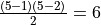 pairings
of other nodes. The normalized betweenness divides the
betweenness by that number to get the average betweenness score
for paths through
pairings
of other nodes. The normalized betweenness divides the
betweenness by that number to get the average betweenness score
for paths through  .
.
Compute the normalized betweenness for the graph in Question 2.
What is the degree centrality of node E in the graph in Question 2?
What is the clustering coefficient for node E in the graph in Question 2?
What is the average path length in the graph in Question 2?
Footnotes