10.2. Introduction to Networkx¶

Note

Most of the points covered here are covered in an ipython notebook (.ipynb). Help with the homework assigned for this module is also available there.

In this section we present a very brief introduction to networkx, one of the more widely used Python tools for network analysis. For the code below to work you must have installed packages named networkx and (for graphviz) pydot. These are part of the standard Canopy distribution.

Some additional networkx help:

For a tutorial on using networkx, look here. Detailed documentation of networkx and many resources and tutorials are available at the Networkx website. But use the Enthought package manager rather than the website for installation.
This Rice University Tutorial. is very stripped down and very well done.

10.2.1. Basics¶

We will import as follows:

>>> import networkx as nx

Networkx provides some graphs as examples. One of these happens to be Zachary’s karate club. That can be read in as follows:

>>> kn=nx.karate_club_graph()

In general, you will be reading in graphs that you construct yourself and save in a file in some standard format or that are available as course data. An alternative way of constructing Zachary’s graph is to download Zachary's karate club network and save this in the directory you start Python in. GML format is a standard graph format networkx knows about, so that file can be read into Python as follows:

>>> kn = nx.read_gml('karate.gml')
<networkx.classes.graph.Graph object at 0x1014b7f90>

You will often find it useful to do:

>>> filename = 'yourfile.gml'
>>> G = nx.read_gml(filename,relabel=True)

The relabel=True flag builds a graph that uses names (actually, whatever occurs as value of the label attribute) as node identifiers. For example, when reading in the Les Miserables graph or the Anna Karenina graph, this will give you characters identified by their two character IDs.

networkx also provides a number of methods that compute statistics of your graph, many of which we will discuss below. To get the number of nodes in your graph, for example, do:

>>> num_nodes = G.number_of_nodes()
>>> print 'number of nodes: ' + str(num_nodes)

10.2.2. Graph generators in `networkx1`¶

Networkx provides a number of functions that generate famous graphs. We have already seen one example. Zachary’s karate club graph can be generated with a simple function call:

>>> kn=nx.karate_club_graph()

To create a Watts-Strogatz (WS) small world graph, do:

>>> G = nx.watts_strogatz_graph(24,4,.3)

G is a WS-graph with 24 nodes, each of which is linked to its four nearest neighbors in the original circular layout. The probability of rewiring is set to .3. Now draw the result.

>>> nx.draw_circular(G)
>>> plt.show()

To create an erdos-renyi graph with 80 nodes, and edge connection probability .1, do:

>>> nx.gnp_random_graph(80,.1)

For more examples of graphs that can be generated, see the Networkx docs.

10.2.3. A simple example¶

As our first example, we will reproduce the result discussed in the visualization section, in which we visualize Zachary’s karate club in a way which that shows the factionalized nature of the social relationships.

First, download Zachary's karate club network and save it in your Python directory, if you haven’t already. Then read it into Python:

>>> kn = nx.read_gml('karate.gml')

You can now draw the graph:

>>> import matplotlib.pyplot as plt
>>> nx.draw_circular(kn)

If you are not working in Ipython with pylab active, you will need to execute the show command to actually display the graph:

>>> plt.show()

You may want to make some small adjustments to the display in the display window. You can then save the figure in an image file in various formats. Here we choose “png”, a standard webbrowser friendly format:

>>> plt.savefig('networkx_circular_karate.png')

10.2.4. Graph analysis¶

networkx has a standard dictionary-based format for representing graph analysis computations that are based on properties of nodes.

We will illustrate this with the example of betweenness_centrality. The problem of centrality and the various ways of defining it was discussed in Section Social Networks. As noted there, key facts about the karate graph can be revealed with a measure of graph centrality called betweenness centrality. networkx offers an implementation, along with a host of other graph analysis tools:

>>> betweenness = nx.betweenness_centrality(kn)

Like the other centrality measures discussed below, betweenness_centrality returns a dictionary associating each node in the graph with a betweenness score. Higher is better. That is, higher means that node is evaluated as occupying a more central position in the graph:

>>> betweenness
{1: 0.43763528138528146, 2: 0.053936688311688304, 3: 0.14365680615680618,
 4: 0.011909271284271283, 5: 0.0006313131313131313, 6: 0.02998737373737374,
 7: 0.029987373737373736, 8: 0.0, 9: 0.05592682780182781, 10: 0.0008477633477633478,
 ...
}

Computing centrality measures is often followed by sorting the results to find the nodes with highest centrality. Here’s an example of how to do that. Dictionaries have no concept of order, so to sort their contents you must first turn them into lists, and then sort the resulting list:

>>> b_il = betweenness.items()
>>> b_il.sort(key=lambda x:x[1],reverse=True)
>>> b_il
[(1, 0.43763528138528146), (34, 0.30407497594997596), (33, 0.14524711399711399),
 (3, 0.14365680615680618), (32, 0.13827561327561325), (9, 0.05592682780182781),
 (2, 0.053936688311688304), (14, 0.04586339586339586), (20, 0.03247504810004811),
 ....
]

So we’ve discovered that node 1 and node 34 have the highest betweenness scores, and might therefore be thought to be the most central people in this social organization, in accord with what is suggested by the display produced by the Fruchterman-Reingold algorithm.

We can compare the results obtained from betweenness_centrality with those from degree_centrality:

>>> deg = nx.degree_centrality(kn)

The results in this case aren’t very different from those of betweenness centrality, so we omit them here.

Other analysis tools implemented in networkx.

edge_betweenness(G): Illustrated below in the the Girvan-Newman example.
eigenvector_centrality(G): (also eigenvector_centrality_numpy). Explaining this concept of centrality is beyond the scope of this course. It requires computing the eigenvectors of the adjacency matrix of the graph, and is closely related to pagerank score used by Google to rank the centrality of websites on the Internet.
nx.closeness_centrality(G). Closeness centrality of a node u is the reciprocal of the sum of the shortest path distances from u to all n-1 other nodes. Since the sum of distances depends on the number of nodes in the graph, closeness is normalized by the sum of minimum possible distances n-1. So if node n is a neighbor of all n-1 other nodes in the graph, closeness_centrality is 1.
current_flow_betweenness_centrality. This kind of centrality was first discussed in [NEWMAN2003] . Newman calls it “random walk centrality”, also known as “current flow centrality”. The current flow centrality of a node n can be defined as the probability of passing through n on a random walk starting at some node s and ending at some other node t (neither equal to n), Newman argues that betweenness for some social networks should not be computed just as a function of shortest paths, but of all paths, assigning the shortest the greatest weight. This is because messages in in such networks may get to where they’re going not by the shortest path, but by a random path, such as that of sexual disease through a sexual contact network.
nx.clustering coefficient(G): clustering(G, nbunch=None, with_labels=False, weights=False) Clustering coefficient for each node in nbunch.
nx.average_clustering(G): Average clustering coefficient for a graph. Note: this is a space saving function ; It might be faster to use clustering to get a list and then take average.
nx.triangles(G, nbunch=None, with_labels=False): Returns number of triangles for nbunch of nodes as a dictionary. If nbunch is None, then return triangles for every node. If with_labels is True, return a dict keyed by node. Note: Each triangle is counted three times: once at each vertex. Note if G is the graph, and t is thenumber triangles of a node n, and d is its degree, then :math: nx.clustering_coefficient(G,n) = frac{t}{d(d-1)}
nx.connected_component_subgraphs(G): Used in the Girvan-Newman implementation below. This returns a list of the fully connected components of graph G. If the graph is fully connected it returns a list containing the graph
nx.number_connected_components(G): This just returns the length of the list returned by nx.connected_component_subgraphs(G).

10.2.5. Implementing Girvan-Newman¶

Here is a simple python implementation of the Girvan-Newman graph-partition method using networkx. The source code is here.

The Girvan-Newman algorithm is divisive. It tries to find an optimal way of cutting the graph into two pieces, and then it does the same on the pieces. Hence the girvan_newman function is recursive. Each time it finds a way to split a graph into two optimal pieces, it calls itself on the pieces. It terminates when it is given a graph with only one node. It returns a list of all the components it has found:

import networkx as nx

def girvan_newman (G):

    if len(G.nodes()) == 1:
        return [G.nodes()]

    def find_best_edge(G0):
        """
        Networkx implementation of edge_betweenness
        returns a dictionary. Make this into a list,
        sort it and return the edge with highest betweenness.
        """
        eb = nx.edge_betweenness_centrality(G0)
        eb_il = eb.items()
        eb_il.sort(key=lambda x: x[1], reverse=True)
        return eb_il[0][0]

    components = nx.connected_component_subgraphs(G)

    while len(components) == 1:
        G.remove_edge(*find_best_edge(G))
        components = nx.connected_component_subgraphs(G)

    result = [c.nodes() for c in components]

    for c in components:
        result.extend(girvan_newman(c))

    return result

Note the use of a while loop in line 21. This keeps removing the remaining edge with highest betweenness. Each time an edge is removed we recompute the edge with highest betweenness as well as the components in the graph. When we get two components, the condition for re-entering the while loop fails, and we exit the loop, having succeeded in splitting the graph. For densely connected graphs, many edges may have to be removed to split the graph.

10.2.6. Using weighted links¶

We read in a weighted version of the karate graph, which has Zachary’s original weights for the intensity of the relationship (this was measured by how many extra-club activities the two club members shared):

import networkx as nx
kn = nx.read_gml('weighted_karate.gml')

Nex we sort the edge list by weight

all_edges = sorted(kn.edges(), key= lambda x: kn.get_edge_data(*x)[0]['value'], reverse=True)

Now for each edge we print the edge and its weight:

from collections import Counter
all_node_ctr = Counter()
for (u,v) in all_edges:
    for x in (u,v):
        all_node_ctr[x] += 1
    print '%-4s %-4s %.3f' % (u,v,weight)

Next we sort by degree:

all_nodes_il = sorted(all_node_ctr.items(), key = lambda x:x[1], reverse=True)
for (char, ct) in all_nodes_il:
    print '%4s  %.3f' % (char, ct)

top_chars_degree_centrality = all_nodes_il[:12]
print
for (ch, ct) in top_chars_degree_centrality:
    print '%4s %.3f' % (ch, ct, )

Now we draw. We’ll use a force-spring layout, and we’ll try increasing spring tension for high weighted edges

new_labels_kn = dict([(char,char) for (char,score) in top_chars_degree_centrality])
pos = nx.spring_layout(kn,scale=1.0,weight='value') #
nx.draw_networkx(kn,pos, with_labels=False,node_size=200,node_color="lightgray")  #Default node size=300
nx.draw_networkx_labels(kn,pos,new_labels_kn,font_size=14,font_color='blue')
nx.draw_networkx_nodes(kn,pos,new_labels_kn,node_color='red',node_size=400,label_pos=1.0,node_shape='D',font_size=16)

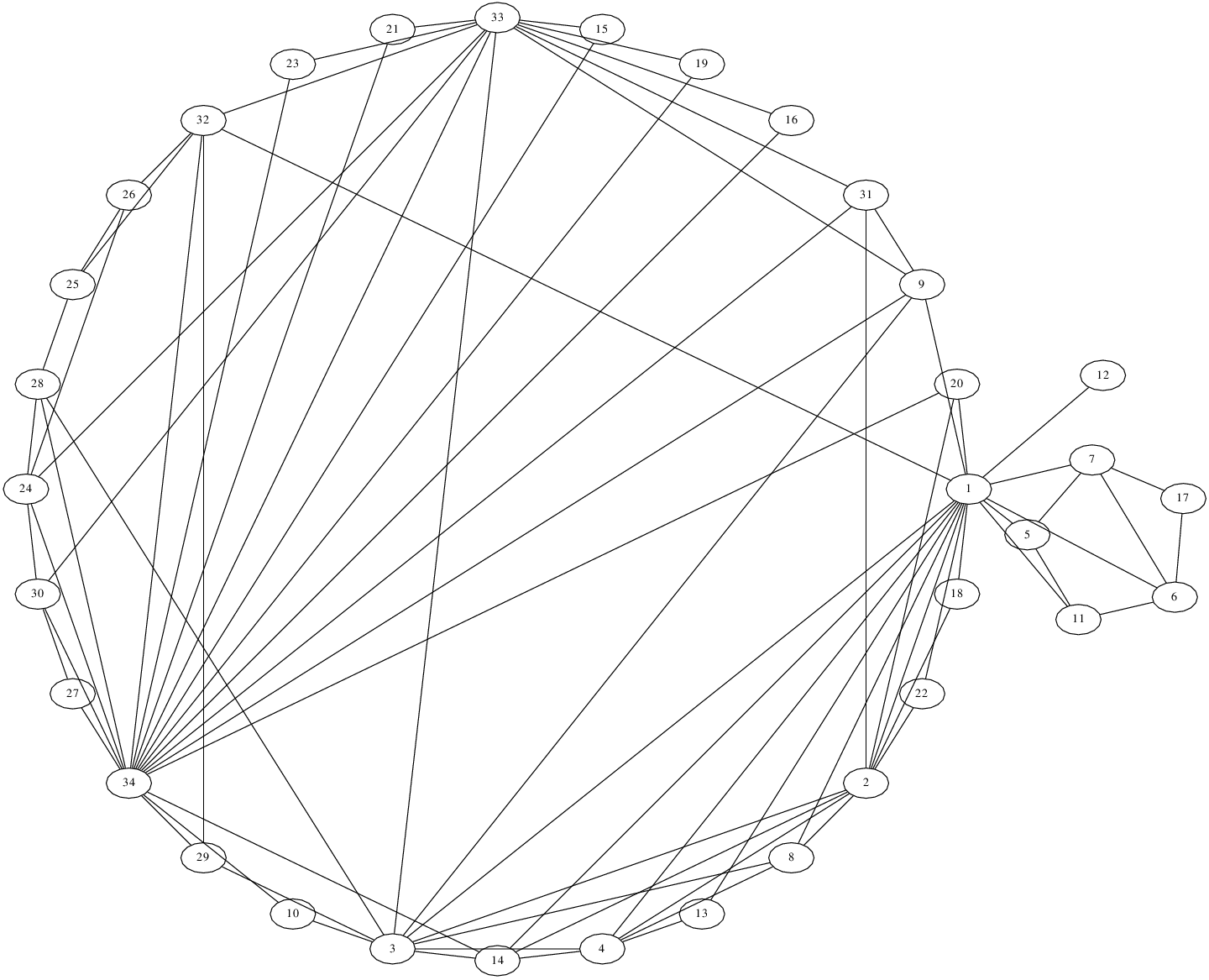
10.2.7. Coloring factions¶

The networkx version of the karate graph has nodes annotated with faction membership information. Let’s use that to color our factions.

The following are the steps taken to produce the colored FG layout figure in the lecture notes. Some of the commented out lines show experiments you could try.

Start with faction1_color as the default node color We make a list of L tokens of the faction1_color string, where L is the length of kn.nodes()

#nx.draw_spring(kn)
#plt.savefig('networkx_spring_karate.png')

import math

#(faction1_col, faction2_col) = ('lightgray','salmon')
(faction1_col, faction2_col) = ('yellow','lightgreen')

node_color = [faction1_col] * len(kn.nodes())
# Now using the faction membership abnnotations from Zachary's data, change the known faction2 nodes to faction2_color.

node_dict = dict(kn.nodes(data=True))
for n in kn.nodes():
    if node_dict[n]['club'] == 'Officer':
        node_color[n] = faction2_col
print node_dict
print node_color

{0: {'club': 'Mr. Hi'}, 1: {'club': 'Mr. Hi'}, 2: {'club': 'Mr. Hi'}, 3: {'club': 'Mr. Hi'}, 4: {'club': 'Mr. Hi'}, 5: {'club': 'Mr. Hi'}, 6: {'club': 'Mr. Hi'}, 7: {'club': 'Mr. Hi'}, 8: {'club': 'Mr. Hi'}, 9: {'club': 'Officer'}, 10: {'club': 'Mr. Hi'}, 11: {'club': 'Mr. Hi'}, 12: {'club': 'Mr. Hi'}, 13: {'club': 'Mr. Hi'}, 14: {'club': 'Officer'}, 15: {'club': 'Officer'}, 16: {'club': 'Mr. Hi'}, 17: {'club': 'Mr. Hi'}, 18: {'club': 'Officer'}, 19: {'club': 'Mr. Hi'}, 20: {'club': 'Officer'}, 21: {'club': 'Mr. Hi'}, 22: {'club': 'Officer'}, 23: {'club': 'Officer'}, 24: {'club': 'Officer'}, 25: {'club': 'Officer'}, 26: {'club': 'Officer'}, 27: {'club': 'Officer'}, 28: {'club': 'Officer'}, 29: {'club': 'Officer'}, 30: {'club': 'Officer'}, 31: {'club': 'Officer'}, 32: {'club': 'Officer'}, 33: {'club': 'Officer'}}
['yellow', 'yellow', 'yellow', 'yellow', 'yellow', 'yellow', 'yellow', 'yellow', 'yellow', 'lightgreen', 'yellow', 'yellow', 'yellow', 'yellow', 'lightgreen', 'lightgreen', 'yellow', 'yellow', 'lightgreen', 'yellow', 'lightgreen', 'yellow', 'lightgreen', 'lightgreen', 'lightgreen', 'lightgreen', 'lightgreen', 'lightgreen', 'lightgreen', 'lightgreen', 'lightgreen', 'lightgreen', 'lightgreen', 'lightgreen']

Next lay out the network:

pos = nx.spring_layout(kn,scale=1.0)

Now put in the labels, using a label->new_label mapping. We’ll change the labels to agree with Zachary’s original indexing, so $x \mapsto x+1$ .

new_labels = dict((x,x + 1) for x in kn.nodes())
nx.draw_networkx_labels(kn,pos,new_labels,font_size=14,font_color='black')

We’ll highlight the two leader nodes, by drawing slightly larger black circles round them. Notice how the edges and nodes have to be drawn separately now.

nx.draw_networkx_nodes(kn,pos,{0:0,33:33},node_color=['black','black'],node_size=800)
# Now draw all the nodes, including leaders, using faction color scheme.
nx.draw_networkx_nodes(kn,pos,new_labels,node_color=node_color,node_size=500)
nx.draw_networkx_edges(kn,pos)

10.2.8. Notes on color¶

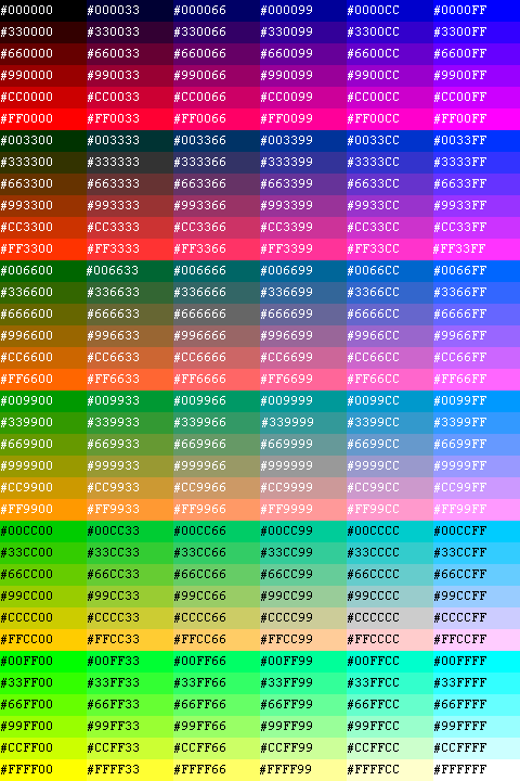
For your choices with matplotlib colors, look here in the matplotlib docs. Or you can use direct html color specs replacing line ?? above with something like this:

>>> (faction1_col, faction2_col) = ('#00CCFF','#FF00FF')

This following table shows the HTML color scheme:

10.2.9. Using the graphviz interface¶

Here is another way to access tools outside of Python for graph drawing, in particular a popular graph drawing program named graphviz.

Via the module pydot networkx provides an interface to graphviz. This is loaded automatically whenever graphviz -relevant functions are called. For example:

>>> nx.write_dot(kn,'networkx_circular_karate.dot')

This writes a “.dot” file. This is a layout neutral representation of the graph. Now graphviz can be called with various layout functions to create an image file from the the graph representation in networkx_circular_karate.dot.

The most interesting result for the karate graph was via the graphviz circo function:

circo -Teps -o networkx_circular_karate_via_dot.eps networkx_circular_karate.dot

The result looks like this.

../_images/networkx_circular_karate_via_dot.png

networkx also offers the option of calling graphviz layout programs directly and plotting them using matplotlib. For example, graphviz ‘s version of a Fruchterman-Reingold layout can be computed as follows:

>>> from networkx import graphviz_layout
>>> layout=nx.graphviz_layout
>>> pos = layout(pb,prog='sfdp')

Then networkx ‘s interface to plotting facilities can be called.