3.3. Python types

We will begin our discussion of basic Python by looking at the builtin Python types.

When you give Python commands it computes things and the results of these computations are most often stored in memory as objects. How objects behave and what kinds of information they represent is determined by their type. There are two kinds of builtin types we need to discuss, simple and compound, roughly equivalent to what computer scientists refer to as scalar types and data structures. For the simple (scalar) case, we’ll begin with numbers, add strings and conclude with Boolean types.

Compound types are data types that can consist of more than one data type, generalpy types that can have other types inside them. For the compound case, we’ll discuss various kind of Python containers, including strings again, because in Python strings are containers. They are not compound because the only type of thing that can be “in” a string is a string, but they are sequences and they are accessed and updated like other sequential containers.There are lots of other types of objects in Python, but these are the most important types for the kinds of computing discussed in this course. In addition, they provide a good starting point for understanding some of the other Python types. Builtin types are a good place to start because learning about types introduces you to certain basic patterns that will be used over and over again in Python; in addition, they teach you how information is represented in Python.   They are not compound because the only type of thing that can be “in” a string is a string, but they are sequences and they are accessed and updated like other sequential containers.

In this section. we discuss two basic kinds of objects in Python, numbers and strings. There are lots of other kinds of objects in Python, but these are the two most important for the kinds of problems discussed in this course.

In addition, they provide a good starting point for understanding some of the other Python types.

3.3.1. Numbers

First, as our first Python session showed, there are numbers:

>>> X = 3

Python actually has several different number types. In many simple scripts, Python programmers do not actually have to think about the different kinds of numbers (this is not true in every programming language!). Nevertheless, it is helpful to understand the basic concept, and since we are going to have to understand how different data types work, it helps to understand how the simplest kinds of type distinctions work, and some of the motivations behind them.

Figure Python number types shows the Python type tree for numbers.

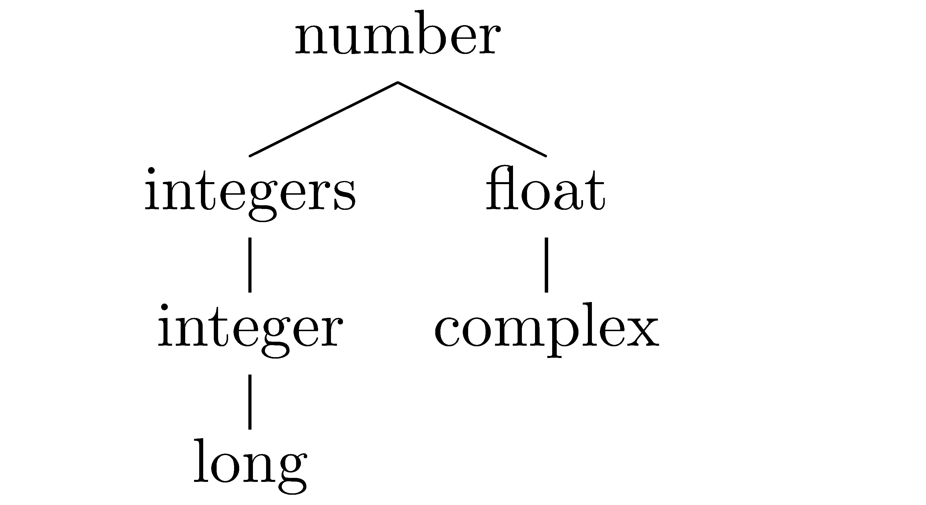
Python number types

Let’s start with the distinction between integers and floats. For most purposes, you can simply think of this as a distinction between the kinds of values you want to represent. For values that are exactly equal to integers (…, -2, -1, 0, 1, 2, …), you use integers (Python type name int); for values that come in between, you use floats:

>>> type(1)
int
>>> type(1.2)
float
>>> X = 1
>>> type(X)
<type 'int'>
>>> X = 1.2
>>> type(X)
<type 'float'>

Now the real question is why bother to have this distinction at all? Why not just have a number type and leave it at that? The answer in part is space. It takes a lot of information to represent values between 1 and 2 exactly. In fact, for many values that come up in mathematics (The value of , for example), it would necessarily take an infinite amount of space. In a decimal representation, fractions like are infinitely repeating decimals, and would also take an infinite of space to represent exactly. Since numbers are represented as binary fractions in computer memory, a different set of fractions comes out as infinitely repeating in computer memory (.1, for example) 1 .

So what we do instead is set aside a standard amount of space for each floating point number we want to use, in fact quite a lot of space — to allow for satisfactory precision in extended calculations. On the other hand, sometimes we don’t want to use numbers for extended mathematical calculations of arbitrary precision. Sometimes we just want to use them for counting. So when I use a particular variable to store the number of times I see the word ricochet, I know that no matter how much data I’ve got, the number of times the word occurs can still be represented by an integer. So for storing an integer we set aside another smaller amount of space, and just as there are floats I can’t represent in the given amount of space, so there are also integers (big ones) I can’t represent in the agreed-upon amount of space. Now if I really need more space, there is another BIGGER data type I can use for REALLY big integers (say I am counting subatomic events), called a long (or long integer), and that too has its limits. When the absolute value of numbers gets too big to represent in the amount of memory available, that’s called overflow.

The opposite problem is numbers that are too small to represent. This state of affairs is equally troublesome, since takes just as much space to represent as ,. When the absolute value of numbers gets too small to represent in the amount of memory available, that’s called underflow.

Finally, there is a distinct number type for complex numbers, which are really numbers with two number components:

>>> X = 3j+2
>>> type(X)
<type 'complex'>

And as you might expect, these take up twice as much space as a float. These come up less in Social Science settings, so we’ll pass over them quickly.

In sum, each of the number data types has its specific purposes, and its specific limits.

Most of these facts aren’t very important in social science computing, but it is important to understand that there are different number types, and that they exist for very good reasons. As the domain of social science computing expands, these kinds of distinctions become important to understand.

For example, since the advent of successful speech recognition systems in the 1980s, the branch of linguistics devoted to computer processing of language has undergone a massive expansion and influx of new ideas. Statistical modeling has become much more important. As a result computing the probabilities of very rare linguistics events (for example rare words such as nuttiness) has become a practical necessity; in such computations, underflow problems often arise, and computational linguists have learned how to write programs that deal with them.

3.3.2. Strings

The other basic data type is strings:

>>> X = 'frog'
>>> type(X)
<type 'str'>

When we type in a word with quotes to the Python prompt, or when we write a program that reads in a file of ordinary English text, generally the data type you get is strings. Unless you tell Python otherwise, the data type you get by reading in a file is strings.

Much of this course will be concerned with dealing with string data, since a lot of data of interest to social scientists is in string form.

The important thing to remember about strings is that when you want to explicitly reference a string value, you need quotes, as in the example above with ‘frog’. Leaving out the quotes is an error:

>>> X = frog
Traceback (most recent call last):
File "<stdin>", line 1, in <module>
NameError: name 'frog' is not defined

Python interprets this as a reference to a variable. The variable frog might refer to anything, an integer, a float, a file; Python doesn’t know; therefore it doesn’t know what value to set X to, and it reports an error.

Python allows any character to occur in a string, including the punctiation marks and spaces. So the following is fine:

>>> X = 'The big dog laughed.'

But how about the quotation mark character? Can that occur in a string? The answer is that it can, but you have to wrap the string in a distinct kind of quotation mark. So both of the following are fine:

>>>  X = "The big dog laughed and said, 'Hello, Jeremy.'"
>>>  Y = 'The big dog laughed and said, "Hello, Jeremy."'
>>>  X == Y
False

The convention is that the string expression has to start and end with the same kind of quotation mark. Any quotation marks inside have to be different and are considered part of the strings being referred to, so X and Y differ in that X contains two instances “’” and Y contains two instances of ‘”’. The quotation marks at the beginning and end of the string are not considered part of the string; they are just delimiters, like parentheses in arithmetic, telling you where the first and last character of the string are. So contrast the above examples with the following:

>>> X = "The big dog laughed."
>>> Y = 'The big dog laughed.'
>>> X == Y
True

Which quotation character you use as your delimiter doesn’t matter (as long as there are no quotation characters inside the string).

Generally speaking, strings of more than one line require some special provisions. They should be begun and ended with triple quotes:

  >>> X = """
  Beautiful is better than ugly.
  Explicit is better than implicit.
  Simple is better than complex.
  Complex is better than complicated.
"""
>>> print(X)

   Beautiful is better than ugly.
   Explicit is better than implicit.
   Simple is better than complex.
   Complex is better than complicated.

Note that the spaces included at the beginning of each line are part of the string. Such multiline strings serve an important purpose in Python, since they are used for documentation.

Strings can also include special characters such as tabs. To place a tab in a string use the special \t symbol; To place a line break in a string use the special \n symbol. Thus, to place a tab between ‘x’ and ‘y’, we write:

>>> Z  = 'x\ty'
>>> print(Z)
x     y

And since \n produces a line break, the string X defined above, giving four lines of the Zen of Python, can also be defined:

>>> X = "\n   Beautiful is better than ugly.\n   Explicit is better than implicit.\n   Simple is better than complex.\n   Complex is better than complicated."
>>> print(X)

Beautiful is better than ugly.
Explicit is better than implicit.
Simple is better than complex.
Complex is better than complicated.

Generally speaking there is little need for multiline strings with explcit \n, except for strings assembled from pieces by a program. The triple-quoted form is preferred because it is more readable.

3.3.3. Other Scalar Types

We haven’t yet talked much about what you can do with scalar types, but once we begin to do things, the need for more basic types becomes evident.

Of course one thing you can do with numbers is arithmetic, as we saw in our brief introduction last chapter, but doing arithmetic on numbers (3 + 2) only result in new numbers (5). What leads to a new type is Boolean tests (tests that return True and False):

>>> 3 > 2
True

>>> 2 > 3
False

Like 3 + 2 and 3*2, 3 > 2 and 2 < 3 are expressions that need to have values that can be used in further computing. These values, printed out here as True and False, are known as Booleans, and Python expressions that have Booleans as their values are generally known as Boolean tests. Other examples of Boolean tests:

>>> x = 3 + 2
>>> x == 5
True

Note that the first line is not a Boolean test; it is an assignment of a value to a name. Not only does it not have a Boolean value. It has no value at all (hence nothing prints out after that line). The second line, on the other hand, is a genuine Boolean test with value True. So now we know two Boolean operators (operation symbols that come between the terms they operate on): < and ==. Other Boolean operators on numbers are: <=, >, >=. Of course == is much more than an operator on numbers. It can be used for comparison of just about any Python types.

Note that True and False are spelled just that way. case matters:

>>> true
NameError: name 'true' is not defined

>>> True
True

Note also that when you correctly enter the name of a known scalar type instance, Python will just evaluate that expression and print out that value in the usual way, meaning it will often print back what you just typed in:

>>> 1
1

So True and 3 > 2 are two expressions whose value is True. We can even test their equality:

>>> (3 > 2) ==  True
True

Of course it would be fairly silly to type this when you can use 3 > 2 to get the same result. Boolean tests will be of particular interest when we get to conditional branching.

The official name of the type is bool:

>>> isinstance(False, bool)
True

Another scalar type is the peculiar Python expression None:

>>> None

Note that by convention, Python actually prints out nothing here. The object None is used in those contexts where a value is called for but no meaningful value exists. For example, suppose we have a kinship database and we write a function spouse that is supposed to return a person’s spouse, What should the function return for unmarried individuals? None is one candidate. Another idea would be to have function return the string "NA" for single people, because that is a completely meaningful answer. But then, what should the function return when applied to a city name or the integer 1? If we are taking "NA" to mean unmarried, that’s the wrong answer. Is the integer 1 unmarried? We might of course throw an exception and halt all computation; but a friendlier alternative is to return None in those cases; that is, None could be what spouse returns when applied to an entity that is clearly out of the function’s intended domain. The general idea is that None is the opposite of a meaningful value. Technically, None is the one and only instance of the type <class 'NoneType'> (this particular type has no convenient name).

Footnotes

1

For an excellent discussion of floats in Python, see this Python tutorial page.