Probabilistic
Context
Free
Grammars
|
|
A probabilistic context free grammar is
a context free grammar with probabilities attached to the rules.
Model Parameters
-
The model parameters are the probabilities assigned
to grammar rules.
Computing Probabilities
-
We discuss how the model assigns probabilities
to strings and to analyses of strings.
Exploiting Probabilities in Parsing
-
We discuss how to find the most probable
parse given the model.
Estimating Parameters
-
We sketch how rule probabilities are estimated from a syntactically
annotated corpus.
|
Probability
Model
|
|
Important Probabilities
-
Rule Probabilities
-
Probability of an expansion given the category being expanded.
P(γ | A), the probability that the sequence of grammar
symbols γ will expand category A. Given the definition
of a conditional probability, this means the probabilities
of all the expansions of a single catgeory must add to 1.
For example:
S -> NP VP, .8 | Aux NP VP, .2
Given that S is being expanded, the probability of the
NP VP rule is .8; the probability of
the Aux NP VP expansion is .2. The rule probabilities
are the parameters of a PCFG model.
Tree Probability
-
The probability of a tree given all the rules used to construct it.
This will be the product of the probabilities of all the rules
used to construct it. We motivate this below.
For now an example. Given this grammar:
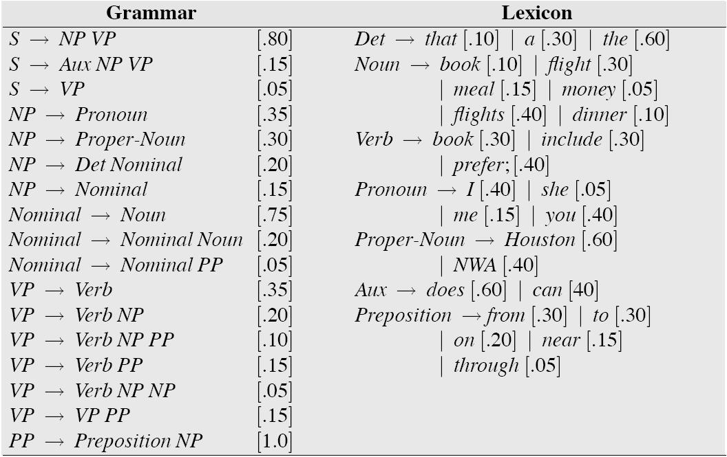
the sentence
Book the dinner flight
has at least two trees:
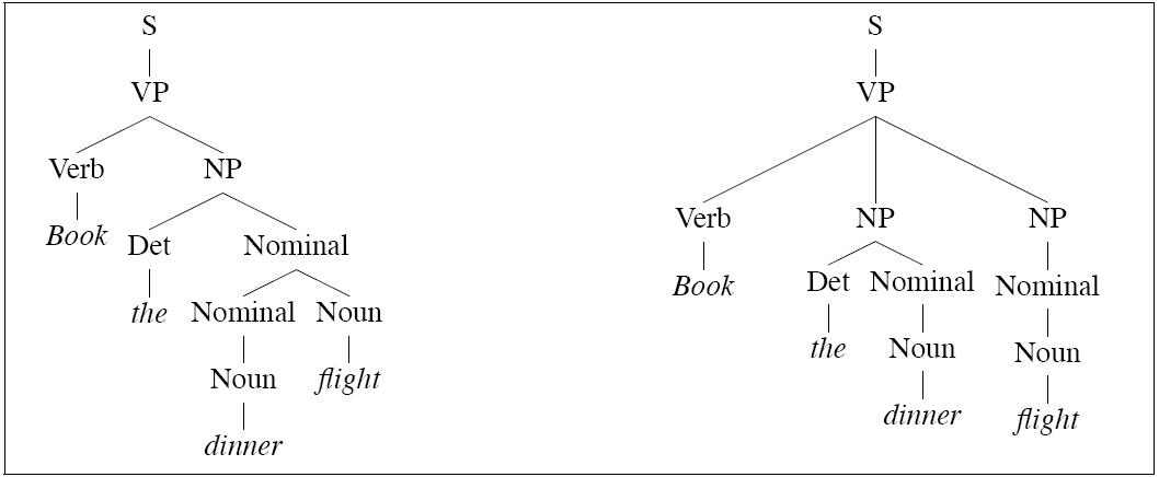
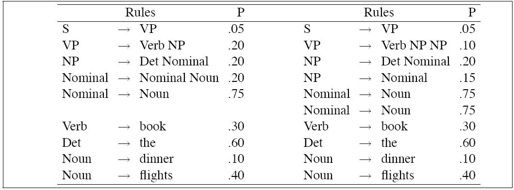
| P(Tleft) | = | .05 * .20 * .20 * .20 * .75 *
.30 * .60 * .10 * .40 = 2.2 × 10⁻⁶ |
|
P(Tright) | = | .05 * .10 * .20 * .15 * .75 *
.75 * .30 * .60 * .10 * .40 = 6.1 × 10⁻⁷ |
Therefore the more probable of the two parses is Tleft,
which is the intuitive result.
String Probability
-
Sum of the tree probabilities for all analyses of the string.
|
Estimating
Parameters
|
|
Given a tree bank,
the maximum likelihood estimate for the PCFG
rule:
VP → VBD NP PP
is:
|
Count(VP → VBD NP PP)
|
|
-----------------------------
|
|
Count(VP)
|
|
Highest
Probability
parse
|
|
Our primary subject of interest is finding
the highest probability
parse for a sentence.
|
This can be done with a rather simple variant of CKY.
CKY is a bottum up algorithm. A bottum up algorithm
is compatible with our probability model because the
probability of a subtree like |
|
|
Is independent of anything outside that tree,
in particular of where that subtree occurs in a sentence
(for instance, subject position or object position),
so once we have found all ways of building a constituent,
we are guaranteed to have found the maximum
amount of probability mass that constituent
can add to any tree that includes it. |
CKY is ideal for our purposes because
no constituent spanning (i,j) is built until
all ways of building constituents
spanning (k,l),
i ≤ k < l < j
have been found. Since we can find the most
probable parses for all possible subconstituents
of a constituent spanning (i,j) before we build
any constituents spaning (i,j), we have the essential
feature of a Viterbi like algorithm.
We modify CKY as follows: instead of building
a parse table in which each
cell assigns value True or False for each
category, we build a parse table in which
each cell assigns a probability to each category.
Each time we find a new way of building an
A spanning (i,j), we compute its probability
and check to see if it is more propbable than
the current value for table[i][j][A].
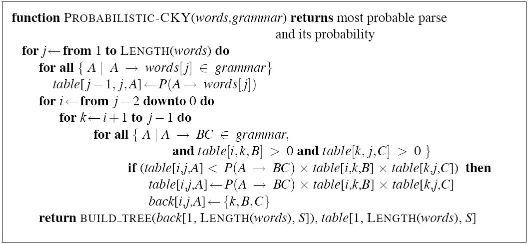
Look here for more
discussion of this Viterbi-like algorithm for finding the
best parse assigned by a PCFG.
|
|
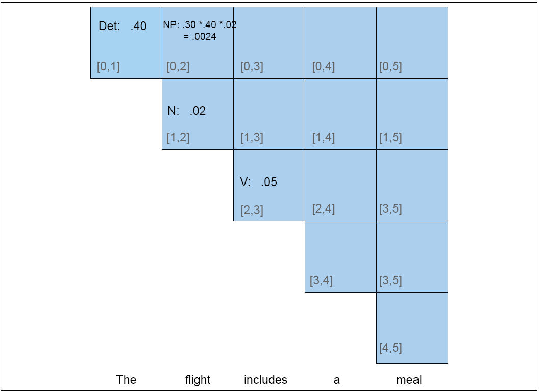
Example
|
|
Partial PCFG:
| S | → | NP VP | .80 |
Det | → | the | .40 |
| NP | → | Det N | .30 |
Det | → | a | .40 |
| VP | → | V NP | .20 |
N | → | meal | .01 |
| V | → | includes | .05 |
N | → | flight | .02 |
|
|
Problems
|
|
Independence assumptions are (damagingly) false
-
Where particular kinds of category expansions
happen very much depends on where in the tree
the category occurs.
Lexical
-
Rule probabilities above the preterminal level are oblivious
to what words occur in the tree. But this is wrong.
|
|
Independence
|
|
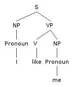
Pronouns (Switchboard corpus [spoken, telephone], Francis et al. 1999)
| | Pronoun | Non-Pronoun |
| Subject | 91% | 9 % |
| Object | 34% | 66% |
|
|
Lexical
|
|
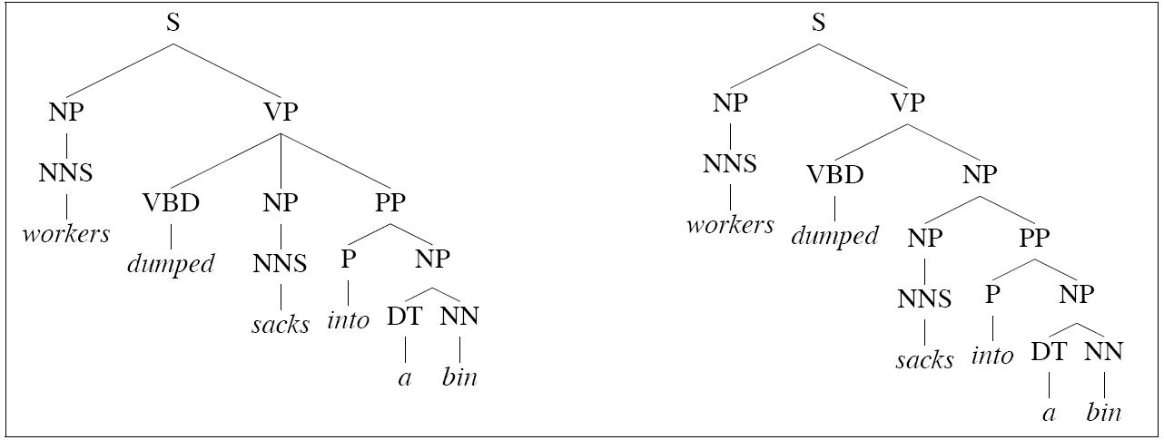
- Left tree is correct for this example
- Right tree is correct for
Conjunction ambiguities can
create trees to which a PCFG cant assign
distinct probabilities, but intuitively,
the tree are quite different in probabilitity:
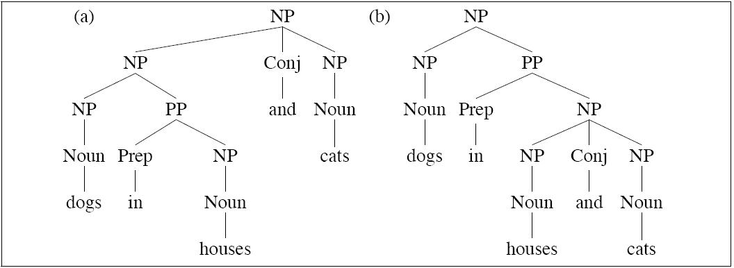
Notice the two trees employ exactly the same bags of
rules, so they must, acording to a PCFG, be equiprobable.
|
Using
grandparents
|
|
Johnson (1998) demonstrates the utility of
using the grandparent node
as a contextual parameter of a probabilistic
parsing model.
This option uses more derivational history.
-
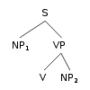
- NP1: P(... | P = NP, GP = S)
- NP2: P(... | P = NP, GP = VP)
Significant improvement on PCFG:
- Can capture distributional differences between subject and
object NPs (such as likelihood of pronoun)
- Outperforms left-corner parser described in
Manning and Carpenter (1997)
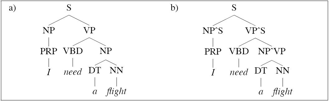
| S → NP VP | | S → NP^S VP^S |
|
|
| NP → PRP | | NP^S → PRP |
| | | NP^VP → PRP |
|
|
| NP → DT NN | | NP^S → DT NN |
| | | NP^VP → DT NN |
This strategy is called splitting. We split the category NP
in two so as to model distinct internal distributions depending
on the external context of an NP Note that in the work
above, preterminals are not split.
|
|
Splitting preterminals
|
|
Johnson's grandparent grammars work because they
reclaim some of the ground lost due
to the incorrectness of the independence assumptions
of PCFGs. But the other problem
for PCFGs that we noted is that they miss
lexical dependencies. If we extend the idea
of gradparent information to preterminals,
we can begin to capture some of that information.
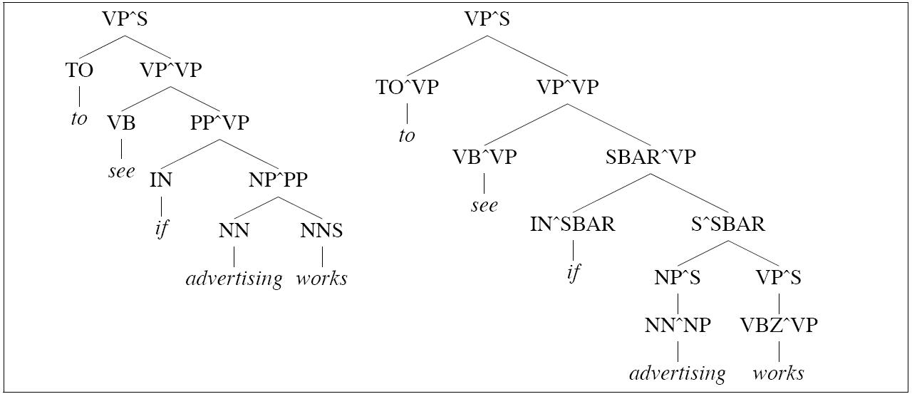
The parse on the left is incorrect because of an incorrect choice
between the following two rules:
PP → IN PP
PP → IN SBAR
The parse on the right, in which the categories (including
preterminal categories) are annotated
with grandparent information, is correct.
The choice is made possible because the string advertising works
can be analyzed either as an SBAR or an NP:
[SBAR Advertising works] when it is clever.
- [NP The advertising works of Andy Warhol]
made him a legend.
Now as it happens words of preterminal category IN
differ greatly in how likely they are to occur with
sentences:
| IN | SBAR |
|
if
| John comes |
|
before
| John comes |
|
after
| John comes |
|
? under
| John comes |
|
? behind
| John comes |
So this is a clear case
where distributional facts about words helps.
And the simple act of extending the grandparent
strategy to preterminals helps capture
the differences between these two classes of IN.
|
Generalized
Splitting
|
|
Obviously there are many cases where splitting helps.
But there are also cases where splitting hurts. We already
have a sparseness problem. If a split results
in a defective or under-represented distribution,
it can lead to overfitting and it can hurt.
Generalizations that were there before the split
can be blurred or lost.
Two approaches:
Hand-tuned rules (Klein and Manning 2003b)
Split-and-merge algorithm: search for optimal splits
(Petrov et al. 2006)
|
Lexicalized
CFGs
|
|
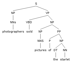
An extreme form of splitting:
| VP → VBD NP PP | |
VP(dumped,VBD) → VBD(dumped,VBD) NP(sacks,NNS) PP(into,P) | |
| | |
VP(sold,VBD) → VBD(sold,VBD) NP(pictures,NNS) PP(of,P) | |
| | |
. . . |
|
|
Notice categories are being annotated with two kinds of information:
- Head word
- Category of their immediately dominated head constituent
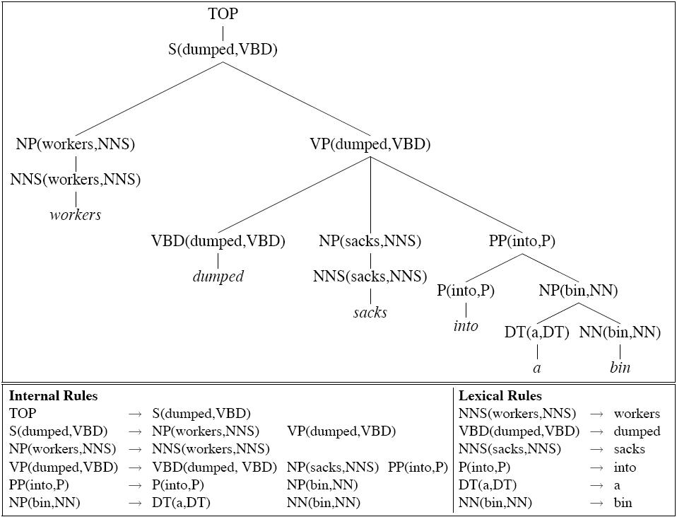
Lexical rules all have probability 1.0
|
Implementing
Lexicalized
Parsers
|
|
Mathematically, a lexicalized PCFG is a PCFG, so
In principle, a lexicalized grammar has an N3 CKY
parser just like any PCFG.
The problem is, we just blew up the grammar when we lexicalized it:
| VP → VBD NP PP | |
| VP(dumped,VBD) → VBD(dumped,VBD) NP(sacks,NNS) PP(into,P) | |
| VP(spilled,VBD) → VBD(spilled,VBD) NP(ketchup,NNS) PP(on,P) | |
| VP(X,VBD) → VBD(X,VBD) NP(Y,NNS) PP(Z,P) | |
And the real parsing complexity is O(n3G2), where G
is the size of the grammar.
The G term now implicitly depends on n or G, whichever is smaller, and n is generally SMALLER than G.
So the real parsing complexity is O(n3n2)
How many distinct attributes can n there now be in a cell for span i,j?
nonterminal, word (between i and j), preterminal of word
Therefore worst case number of items in a span:
num nonterminals X n (num words between i and j) X num poses
If we assume every part of speech can "project" only one non terminal:
|Nonterminals| X n
That's how many distinct floating point numbers (probs) we may need to store for a span (a cell
in the table).
Data structures?
Currently a cell is filled buy a dictionary from nonterminals to floats.
table[3][5] = {NP: .003, VP: 0004}
What shd replace it?
Answer:
A dictionary from a pair of nonterminals and words to floats.
{(NP,sacks): .003, (VP,sacks): .0004, (VP,dump):.01}
Note: At the same time, a lexicalized grammar rule may look like this:
(NP, sacks) → sacks 0.01
(VP, helps) → (VBZ,helps) (NP,students) 0.0001
|
Making
a lexicalized
grammar
|
|
VP → VBD NP .1
VP → VBD .9
VBD → kicked .1
VBD → saw  .8
VBD → drank .1
NP → Det N  1.0
Det → a  .2
Det → the .8
N → book  .1
N → ball  .7
N → gin  .2
Then the lexicalized grammar with uniform probabilities is:
S → (NP,book) (VP,kicked) .111
S → (NP,book) (VP,kicked) .111
S → (NP,book) (VP,kicked) .111
 S → (NP,gin) (VP,kicked) .111
S → (NP,gin) (VP,kicked) .111
S → (NP,gin) (VP,kicked) .111
 S → (NP,ball) (VP,kicked) .111
S → (NP,ball) (VP,kicked) .111
S → (NP,ball) (VP,kicked) .111
(VP,kicked) → (VBD,kicked) (NP,book) .033
(VP,kicked) → (VBD,kicked) (NP,gin) .033
(VP,kicked) → (VBD,kicked) (NP,ball) .033
(VP,kicked) → (VBD,kicked)  .3
(VP,kicked) → (VBD,kicked)  .3
(VP,kicked) → (VBD,kicked)  .3
(VP,saw) → (VBD,saw) (NP,book) .033
(VP,saw) → (VBD,saw) (NP,gin) .033
(VP,saw) → (VBD,saw) (NP,ball) .033
(VP,saw) → (VBD,saw)  .3
(VP,saw) → (VBD,saw)  .3
(VP,saw) → (VBD,saw)  .3
(VP,drank) → (VBD,drank) (NP,book) .011
(VP,drank) → (VBD,drank) (NP,gin) .011
(VP,drank) → (VBD,drank) (NP,ball) .011
(VP,drank) → (VBD,drank)  .3
(VP,drank) → (VBD,drank)  .3
(VP,drank) → (VBD,drank)  .3
(VBD, kicked) → kicked 1.0
(VBD,saw) → saw  1.0
(VBD,drank) → drank 1.0
(NP,book) → (Det,a) (N,book)  .5
(NP,book) → (Det,the) (N,book)  .5
(NP,ball) → (Det,a) (N,ball)  .5
(NP,ball) → (Det,the) (N,ball)  .5
(NP,gin) → (Det,a) (N,gin)  .5
(NP,gin) → (Det,the) (N,gin)  .5
(Det,a) → a  1.0
(Det,the) → the 1.0
(N,book) → book  1.0
(N,ball) → ball  1.0
(N,gin) → gin  1.0
|
Sparseness
problems
|
|
Maximum likelihood estimates for the PCFG defined
by lexicalized splitting are doomed by sparseness:
The rule prob for:
| VP(dumped,VBD) → VBD(dumped,VBD) NP(sacks,NNS) PP(into,P) | |
is:
|
Count(VP(dumped,VBD) → VBD(dumped,VBD) NP(sacks,NNS) PP(into,P))
|
|
-----------------------------------------------------------
|
|
Count(VP(dumped,VBD))
|
No corpus is likely to supply reliable counts for such events.
How do we usually solve sparseness problems?
We need to make some further independence assumptions!
|
|
Collins I
|
|
Generation story: Break down a rule into number
of contextually dependent subevents which collectively "generate"
an occurrence of a rule:
LHS → Ln Ln-1 ... H R1 ....
Rn-1 Rn
Basic decomposition: Generate head first, then Li
modifers terminating with STOP, then Ri modifiers
terminating with STOP. For the tree above we have the following
sub event probs
- P(H|LHS) = P(VBD(dumped,VBD) | VP(dumped,VBD))
- Pl(STOP | VP(dumped,VBD), VBD(dumped,VBD))
- Pr(NP(sacks,NNS) | VP(dumped,VBD),VBD(dumped,VBD))
note independent of any left modifiers
- Pr(PP(into,P) | VP(dumped,VBD),VBD(dumped,VBD)):
note independent of NP(sacks,NNS)
- Pr(STOP | VP(dumped,VBD), VBD(dumped,VBD),PP)
Let
R = VP(dumped,VBD) → VBD(dumped,VBD) NP(sacks,NNS) PP(into,P))
We estimate the probability of R
by multiplying these probs together:
P(R) =
P(VBD(dumped,VBD) | VP(dumped,VBD)) ×
Pl(STOP | VP(dumped,VBD), VBD(dumped,VBD)) ×
Pr(NP(sacks,NNS) | VP(dumped,VBD),VBD(dumped,VBD)) ×
Pr(PP(into,P) | VP(dumped,VBD),VBD(dumped,VBD)) ×
Pr(STOP | VP(dumped,VBD), VBD(dumped,VBD),PP)
|
|
State of the art
|
|
Using the PARSEVAL metric for comparing gold standard
and system parse trees (Black et al. 1991),
state-of-the-art statistical parsers trained on the Wall
Stree Journal treebank are performing
at about 90% precision 90% recall.
|