2.4.2. Running python in the cloud¶

The option we will discuss here is the Google Colab notebooks. Google colab notebooks are based in many ways on Jupyter notebooks (discussed in the next section), which are in turn extended from IPython.

Google colab notebook is another way of interacting with python, just like IPython is, but Google colab notebook uses your browser, has a very natural command interface, and makes an editable record of your Python session as you go. Commandwise, Google Colab notebooks are an extension of IPython, so for those of you have used IPython, the notebooks will feel very natural. If you’ve used Jupyter notebooks to work with local copies of a notebook, things should feel especially natural. You can freely switch back and forth between Colab notebooks and Jupyter notebooks because the notebooks are save in identical file formats. Throughout this course whatever I say about using a python notebook will apply to either Jupyter notebooks or Google Colab notebooks.

The key difference between using a Jupyter notebook and a Google colab notebook is that the colab notebook is running on some Python server on the cloud. You do not need to have python on your machine to interact with the notebook. In fact the version of python currently available through Google colab seems to have almost all the basic modules we’ll be using in this course. Where that’s not true, the notebook includes some code for installing the module you need in your Python cloud image.

There is plenty of excellent help available for using colab notebooks on the colab.research.google.com website. You can start with this introductory tutorial. In addition, the example notebooks under either the Classic notebook icon or the Jupyter Lab icon on the Jupyter notebook pages on the jupyter.org website are all compatible. As an extra bonus most of the documentation of features in IPython notebook will also work in Jupyter notebook, for example, Chapter One of the Python Data Science Handbook (2017, Jake VanderPlas, O’Reilly).

In the remainder of this section we’ll discuss how to get this magic to happen. First you will access notebooks through links, either from modules on Canvas or from online chapters of this book. Here is your first notebook link.

If you clicked on this link you were taken to a page hosted by google colab, which runs notebook that have been posted on a project management/software collaboration site called github. One advantage of storing software tools on a site like github is that a certain amount of identity checking and exposure is involved; another is that software collaboration tools are implemented, such as version branching and version control. For our purposes, the main benefit is that Google likes github. What you’re looking at when you visit the link is a notebook running Python that you can interact with.

On the other hand if you try this link to the same notebook what you visit is a rendering of the notebook, often a pretty good one that will be suitable for purposes of discussion. But what you won’t be able to do unless you do some customizing is interact with the notebook. By that I mean: Type a python command and have something happen. The difference between the two links is the domain. The link that gives a notebook you can interact with takes you to colab.research.google.com/github.com/gawron, while the other link takes you to my github repository github.com/gawron. The latter domain is also where you will end up if you do a Google search on Gawron github. Even though you can’t interact with the notebooks in the github.com/gawron repository, there is actually some usefulness to visiting the repository since it hosts all the notebooks used in this course. Once there, if you do find you want to interact with a particular notebook, it is relatively easy.

Here are two ways. First, open the Github notebook that you want to work with on github. Typing in the URL address window located at the top of your browser, change the domain from ‘github.com’ to ‘githubtocolab.com’. Reload. The notebook will open in Colab.

The second way to interact with a github notebook is to use a browser that has an “Open in Colab” addon. One such browser is of course Google Chrome. To get the Chrome addon, do the following:

Run Google Chrome as your browser (for this python session), which may require installing it if you don’t have it: Google Chrome install link.

Install the “Open in Colab” extension (just needs to be done once).

Follow a link to a github notebook page (like this one). and wait until the notebook finishes rendering (which can sometimes take a few seconds with some of the longer notebooks).

Click on your “Run in colab” button (now attached to your browser menu bar). The logo looks like this:

At some point before you actually run the notebook and get some output, you will be required to be logged in to your Google apps account (the same account that hosts your Gmail and your Google Drive).

That’s it. One way or another you are now running a Python notebook for thjis course in the cloud and interacting with it. You can import new Python modules, load data, and run analysis code. Everything discussed in this text that involves interacting with Python or interacting with a notebook should work. You can also save your notebook to your own machine or to Google Drive and interact with a local copy on your computer. If you save it to your own machine and you want to run it there, you need to habe Python installed on your local machine and you should read the next section and learn about using Jupyter notebook, because that’s what you’ll be using. Note: there is also a Firefox addon that lets you run notebooks in Google Colab here.

Once you have a notebook running interactively, you can follow along with everything happening in a live lecture and have an updated record of the effects. If something doesn’t work as advertised, you can raise the issue right away.

For accessing data we will be using one of three strategies:

Load the data into the notebook each time you start it from off the web.

Load data from your Google Drive. This is if you’re running in Google Colab. It is very easy to mount your Google Drive while running a Google Colab notebook (there is a clickable widget for doing this).

Save data to your local machine and load it while running Jupyter Notebook.

For more discussion about ways to import data in a Google Colab: notebook, see this article

Another way of running any of the course notebooks in the cloud us suggested by this tutorial.

Open https://nbviewer.jupyter.org/. Enter the github URL of the course notebook you want to run, for example https://github.com/gawron/python-for-social-science/blob/master/numpy/numpy.ipynb. The notebook ill open in noninteractive mode, much as it does on github. However, it will appear with the title Jupyter nbviewer and in the upper hand corner of thedisplay, you will see several icons. Hover over these until you find one that has three intersecting rings and its description will read “Execute on binder.” Click on that and you wil get an interactive version of the notebook.

2.4.3. Starting up python¶

This section assumes you have installed Python. As discussed above, that’s only for people who’ve decided they want to install python; that is, they don’t always want to run in the cloud.

The first thing some of you will want to do is to point and click at something to start Python.

Try not to do this at first. The problem is that the programs that installed Python may have done something to help you start up Python, but often the particulars of how that works are hard to get at. We would like to have as much control with how Python is run as possible. And we want to be able to know what window to look in to see the things a Python program prints out. This helps enormously in knowing what to do when something goes wrong.

Therefore, we are going to start Python from the commandline.

The following notes basically give you three ways to start up Python:

Giving the python command at a command window.
Using IPython
Using Jupyter notebook or Google colab

Version 3 is the recommended version for the first part of the course, but the first time you run Python you should try all three versions in the order given above to verify that

Python is installed correctly (if you installed it)
IPython is installed correctly.
Your browser works with Jupyter notebook and Google Colab.

Ultimately, you will find all 3 ways of starting up Python useful, since they provide a way of interacting with Python that can be useful.

2.4.3.1. Commandline startup: Version I¶

From the commandline means you need to start a Terminal or an MSDos command window that allows you to type commands directly into it. In MacOS X, the default terminal program is called Terminal (From the Go Menu, select Utilities > Terminal); In Windows, it is is called MSDos (From the Start Menu, select Programs > MSDos Prompt).

Windows terminal¶

MacOSX Terminal¶

For Windows 8+ users, the following may help (from ComputerHope.com):

From the Start screen type cmd and press enter; OR
Move the mouse cursor to the very bottom-left corner of the screen and right-click or press Windows key + X. This will open the power user task menu, select either Command Prompt or Command Prompt (Admin).

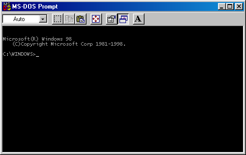
2.4.3.2. The Python command: Windows¶

On Windows machines, the Python installation is usually placed in C:\Python36, though you can change this when you’re running the installer.

If python is installed in one of the usual places Windows looks for programs, the following command (issued in an MSDOS or Command window):

C:\Windows> python

will start up Python, which should look something like this:

Python 3.6.5 |Anaconda, Inc.| (default, Apr 26 2018, 08:42:37)
>>>

Try typing something at the “>>>” prompt:

>>> print ('hello')
hello

Python responds by printing ‘hello’, with no quotes. If the command is unknown, see the next section.

The program you are interacting with when you type commands to the “>>>” prompt is called a python shell. The interactive capability of Python is one of its most important features as a programming language, and one of the features that is most useful for beginners.

Throughout these notes, when indicating terminal commands (as opposed to commands to Python), we will assume a user named gawron whose home directory name (gawron) is printed out in the Terminal window as a prompt.

Typing an end-of-file character (Control-Z on Windows) at the primary prompt causes the shell to exit. If that doesn’t work, you can exit the interpreter by typing the following command: quit().

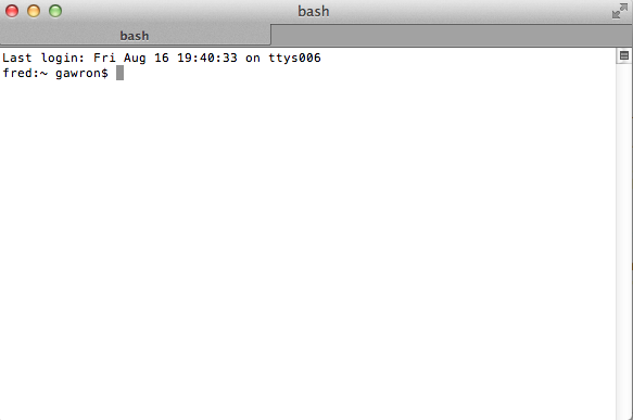
2.4.3.3. The Python command: MacOSX, Unix¶

With a normal Python install on MacOSX, you should just be able to type Python to a terminal window to start python (Terminal application Go > Utitlities> Terminal):

That is:

~ gawron$ python

should start up Python, which looks like this:

Python 3.6.5 |Anaconda, Inc.| (default, Apr 26 2018, 08:42:37)
[GCC 4.2.1 Compatible Clang 4.0.1 (tags/RELEASE_401/final)] on darwin
Type "help", "copyright", "credits" or "license" for more information.  Python 2.7.2 (default, Oct 11 2012, 20:14:37)
 >>>

Try typing something at the “>>>” prompt:

>>> print ('hello')
hello

Python responds by printing ‘hello’, with no quotes.

The program you are interacting with when you type commands to the “>>>” prompt is called a python shell. The interactive capability of Python is one of its most important featurs as a programming language, and one of the features that is most useful for beginners.

Throughout these notes, when indicating terminal commands (as opposed to commands to Python), we will assume a user named gawron whose home directory name (gawron) is printed out in the Terminal window as a prompt.

Typing an end-of-file character (Control-D on Unix and MacOSX, Control-Z on Windows) at the primary prompt causes the Python shell program to exit. If that doesn’t work, you can exit the program by typing the following command: quit().

2.4.3.4. The Python command: Troubleshooting (Windows, MacOSX, Unix)¶

The instructions in this section should help you get python starting up in a command window, if that isn’t working on your machine. Following these instructions will also help you get IPython and jupyter notebook working in a command window.

If you installed the Anaconda version of Python, starting up Python in a command window should look something like this:

fred:Introduction gawron$ python
Python 3.6.5 |Anaconda, Inc.| (default, Apr 26 2018, 08:42:37)
>>>

The information printed out may differ in details such as the version number, but the first line should be the same; it should mention “Anaconda.” If you installed Anaconda Python and you get an error such as “python: command not found” or python starts, and you don’t see any information mentioning “Anaconda” appearing, there are two possibilities:

There is something wrong with the Anaconda installation.
Your machine isn’t finding the right version of Python when you type python in a terminal window.

You can eliminate the first possibility by starting Anaconda Navigator (which is installed as a separate Application along with your Anaconda python). The Navigator startup window looks like this:

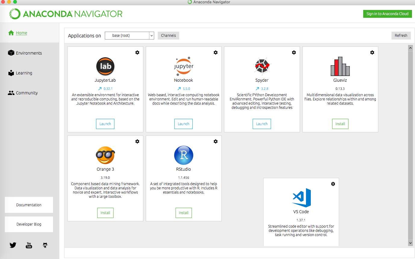
../_images/anaconda_navigator_startup.png

Click on the Spyder application and when the new window appears, select the window labeled IPython Console. After typing some code and typing enter, there will be some output in that window. For example, if we type:

print (True)

in the IPython console, the IPython window will look like this:

Python 3.6.5 |Anaconda, Inc.| (default, Mar 29 2018, 13:14:23)
Type "copyright", "credits" or "license" for more information.

IPython 6.4.0 -- An enhanced Interactive Python.

In  [1]  print(True)
Out [1]  True

Ok, so we are running Python. This means that the Anaconda installation is working. If starting up Python via Anaconda Navigator doesn’t work, you need to get back in touch with Anaconda and find out what wrong with the installation process.

We turn here to investigating possibility 2, that the commandline window is not properly set up to find the Anaconda installation of Python. Input the following commands into a Ipython window window (possibly started via Navigator) and run it:

import sys
print (sys.path)

This program prints the value of the name sys.path. The output in the Ipython window might look like this:

'', '/Users/gawron/anaconda3/lib/python36.zip',
    '/Users/gawron/anaconda3/lib/python3.6',
    '/Users/gawron/anaconda3/lib/python3.6/lib-dynload',
    '/Users/gawron/anaconda3/lib/python3.6/site-packages',
    '/Users/gawron/anaconda3/lib/python3.6/site-packages/aeosa',
    '/Users/gawron/anaconda3/lib/python3.6/site-packages/IPython/extensions',       '/Users/gawron/.ipython']

sys.path is a list of the locations on your computer in which the Anaconda installation looks for Python modules and programs. Look at the second entry in the list, a long path which ends with lib/python3.6. Call the part of this this long path that comes before lib/python3.6 $PYTHONHOME. In the example above, the value of $PYTHONHOME is:

/Users/gawron/anaconda3/

Most of the other entries in sys.path are continuations of $PYTHONHOME. Some of these locations are specific to a Mac; others (such as site-packages) will show up in any Python.

Having determined the value of $PYTHONHOME, you know know the location of the Anaconda python program. It is in $PYTHONHOME/bin. That is, you can now start up a command window, and start the right python by cutting and pasting the value of $PYTHONHOME into it, and following that location with “bin/python”. So for example, on my machine, with the above value for $PYTHONHOME, the complete command line is:

gawron$ /Users/gawron/anaconda3/bin/python

If you hit return after entering this, you get the correct Python startup messages:

Python 3.6.5 |Anaconda, Inc.| (default, Apr 26 2018, 08:42:37)
[GCC 4.2.1 Compatible Clang 4.0.1 (tags/RELEASE_401/final)] on darwin
Type "help", "copyright", "credits" or "license" for more information.
>>>

So now we know how to start up the right version of python on your machine. Of course this is too much to type each time. What you need to do next is add the value of $PYTHONHOME/bin to your PATH, the list of places your command window looks when it starts up programs. The correct procedure for doing this varies from platform to platform.

Let’s start with most Mac and Linux based machines. There is a file executed every time you start a command window, which we can use to set the value of path. This is in your home directory (‘/Users/gawron’ for me) and is called “.bash_profile” (note the name starts with a “.”). Note: every time you start a new command window, it is connected to your home directory.

What you need to do is edit that file with a plain text editor such as pico <https://www.ccsf.edu/Pub/Fac/pinepico.html>-, emacs, vi, or TextWranger. and add the following line:

export PATH=/Users/gawron/anaconda3/bin:$PATH

This adds $PYTHONHOME/bin to $PATH and also preserves and existing values that were already there. If a file named “.bashrc” does not alredy exist in your home directory, that’s fine, create one, and insert just the above line. Under no circumstances should you use Microsoft Word to do your editing. Although Word has something called a “Save as Text” option, the designers were unable to resist the temptation to add idiosyncratic features that make the saved files unusable by other programs. The editors pico, vi and emacs all exist pre-installed on most Mac and Unix systems. You can run them by typing the command name followed by the file name in a command window; pico is by far the easiest to use, and should work fine for this task. So to edit “.bash_profile” with pico, we would start up a fresh command window and type:

gawron$ pico .bash_profile

For Windows users, the concept of a path also exists, and the fix is the same. You have to find out what your $PYTHONHOME folder is (as done above) and add $PYTHONHOME/bin to the path. In changing the path, be sure that you only add a location; don’t delete any locations that are already there. For extra info do a Google search on Windows X.X changing PATH, replacing X.X with your own version of Windows as needed.

2.4.3.5. Commandline startup: IPython¶

If you installed the Anaconda version of Python, you got IPython along with it. And you can start up python with much more helpful set of tools available by typing:

~ gawron$ ipython

This starts up a Python shell with all the resources of a normal Python shell, plus some others. See the IPython website for a quick tour.

If you did not install the Anaconda Python distribution, you can install IPython separately. by going to IPython.org.

The default directions will tell you to install IPython by installing Anaconda. If you have reasons not to do this, you will have to follow the more complicated detaled instructions here.

Many of the scripts we will talk about involve displaying some sort of plot of your data. You will find that all those scripts run more smoothly if run through IPython with its pylab plotting interface set up. This is done by calling:

~ gawron$ ipython --pylab

when starting up IPython. What this does is set up an interface with a windows manager so that plots can be launched authomatically during the session. This is optional; the advantage is that when the same plot programs are run directly through a normal python shell, the interactive shell is frozen while the plot window is up, so that you can’t administer Python commands while continuing to look at the plot. Interaction can be restored by killing the plot window.

A routine IPython startup looks like this:

 gawron$ ipython --pylab

Python 3.6.5 |Anaconda, Inc.| (default, Apr 26 2018, 08:42:37)
Type 'copyright', 'credits' or 'license' for more information
IPython 6.4.0 -- An enhanced Interactive Python. Type '?' for help.
Using matplotlib backend: MacOSX

In [1]:

In [1]: print ('hello')
hello

Throughout these course materials we will use both standard python sessions and IPython sessions. Students are encouraged to use IPython whenever possible (or the Anaconda graphical-user interface which includes IPython), but are warned that some graph-plotting commands may not work quite the same way in standard python as they do in IPython. See Section pandas_introduction.

2.4.3.6. Commandline startup: Jupyter notebook¶

For the first part of the course, the recommended way to work on an assignment is to use Jupyter notebook pages (or equivalently, Colab notebooks, discussed above, for those running in the cloud).

Jupyter notebook is really just another way of interacting with python, just like IPython is, but Jupyter notebook uses your browser, has a very natural command interface, and makes an editable record of your Python session as you go (you will have to remember to save your session). Commandwise, Jupyter is an extension of IPython, so for those of you have used IPython, the Jupyter notebooks will feel very natural. There are also numerous examples on the Jupyter notebook pages on the jupyter.org website. As an extra bonus much of the documentation of features in IPython notebook will also work in Jupyter notebook, for example, Chapter One of the Python Data Science Handbook (2017, Jake VanderPlas, O’Reilly).

You start Jupyter notebook either with Anaconda Navigator or in a command window as follows:

gawron$ jupyter notebook

If you want the pylab interface (for plotting graphs) you do:

gawron$ jupyter notebook  --pylab

The key idea is that this a combination editing environment and Python interpreter. First you break your programming task down into steps. For each step you do the following:

You can write some code, execute it, see the results, edit the code, and repeat until the results look right.

Then you can move on to on to another step. When you have completed all the steps in an assignment, you can save your results as a notebook, a special kind of document any one with IPython can run, and turn that notebook in.

Using the notebook gets you used to a write/execute/edit loop that scales right up to the way real data scientists work. Have a look at this blog post by a data scientist named Philip Guo describing how the Notebook changed the way he worked (written back when jupyter notebook was called ipython notebook).