Probabilistic Context-Free Grammars

Probabilistic
Context
Free
Grammars
A probabilistic context free grammar is a context free grammar with probabilities attached to the rules.

Model Parameters
The model parameters are the probabilities assigned to grammar rules.

Computing Probabilities
We discuss how the model assigns probabilities to strings and to analyses of strings.

Exploiting Probabilities in Parsing
We discuss how to find the most probable parse given the model.

Estimating Parameters
We sketch how rule probabilities are estimated from a syntactically annotated corpus.

Probability
Model

Important Probabilities

Rule Probabilities
Probability of an expansion given the category being expanded. P(γ | A), the probability that the sequence of grammar symbols γ will expand category A. Given the definition of a conditional probability, this means the probabilities of all the expansions of a single catgeory must add to 1. For example:
S -> NP VP, .8 | Aux NP VP, .2
Given that S is being expanded, the probability of the NP VP rule is .8; the probability of the Aux NP VP expansion is .2. The rule probabilities are the parameters of a PCFG model.

Tree Probability
The probability of a tree given all the rules used to construct it. This will be the product of the probabilities of all the rules used to construct it. We motivate this below.
For now an example. Given this grammar:

the sentence
Book the dinner flight
has at least two trees:

P(T_left) = .05 * .20 * .20 * .20 * .75 * .30 * .60 * .10 * .40 = 2.2 × 10^-6

P(T_right) = .05 * .10 * .20 * .15 * .75 * .75 * .30 * .60 * .10 * .40 = 6.1 × 10^-7

Therefore the more probable of the two parses is Tleft, which is the intuitive result.

String Probability
Sum of the tree probabilities for all analyses of the string.

Estimating
Parameters

Given a tree bank, the maximum likelihood estimate for the PCFG rule:
VP → VBD NP PP
is:

Count(VP → VBD NP PP)

-----------------------------

Count(VP)

Real
WSJ data
The sentence below
python -i print_penn_trees.py penn_example.mrg 0

(Start (S (NP (NNP Rolls-Royce) (NNP Motor) (NNPS Cars) (NNP Inc.)) (VP (VBD said) (SBAR (-NONE- 0) (S (NP (PRP it)) (VP (VBZ expects) (S (NP (PRP$ its) (NNP U.S.) (NNS sales)) (VP (cat_TO to) (VP (VB remain) (ADJP (JJ steady)) (PP (IN at) (NP (QP (IN about) (CD 1,200)) (NNS cars))) (PP (IN in) (NP (CD 1990)))))))))) (cat_. .)))

Real
WSJ rules Lexical

Below we present a TINY extract of the rule counts from the WSJ corpus.
2 VBZ --> grants 2 VBZ --> grinds 2 VBZ --> gripes 2 VBZ --> groans 2 VBZ --> halts 2 VBZ --> hands 2 VBZ --> harbors 2 VBZ --> hates 2 VBZ --> heats 2 VBZ --> hosts 2 VBZ --> houses 2 VBZ --> ignores 2 VBZ --> industrials 2 VBZ --> irritates 2 VBZ --> jeopardizes
Propernames in particular
1 NNP --> JKD 1 NNP --> JPI 1 NNP --> JROE 1 NNP --> JUMPING 1 NNP --> Jaap 1 NNP --> Jacki 1 NNP --> Jaclyn 1 NNP --> Jacobsen 1 NNP --> Jacqueline 1 NNP --> Jacques-Francois 1 NNP --> Jaime 1 NNP --> Jakarta 1 NNP --> Jakes 1 NNP --> Jalaalwalikraam 1 NNP --> Jalalabad 1 NNP --> Jamieson 1 NNP --> Janeiro 1 NNP --> Janice 1 NNP --> Janlori 1 NNP --> Janney 1 NNP --> Jansen 1 NNP --> Jansz. 1 NNP --> Japan-U.S
Non-lexical
1 NP --> NNP ''_cat NNP POS 1 NP --> NNP ,_cat 1 NP --> NNP ,_cat CD 1 NP --> NNP ,_cat CD ,_cat CD 1 NP --> NNP ,_cat NNP ,_cat NNP ,_cat NNP ,_cat NNP ,_cat NNP ,_cat NNP CC NNP 1 NP --> NNP ,_cat NNP ,_cat NNP ,_cat NNP ,_cat NNP CC NNP 1 NP --> NNP ,_cat NNP ,_cat NNP NNP CC NNP 1 NP --> NNP ,_cat NNP CC NNP ._cat 1 NP --> NNP ,_cat NNP CC NNP NN NNP NNP 1 NP --> NNP ,_cat NNP CC NNP NNP NNS 1 NP --> NNP ,_cat NNP CC NNPS 1 NP --> NNP ,_cat NNP CC RB NNP 1 NP --> NNP ,_cat NNP NNP ._cat 1 NP --> NNP ,_cat NNP NNP CC NNP NNP 1 NP --> NNP ,_cat NNPS CC NNP NNP 1 NP --> NNP ,_cat RB NN ,_cat 1 NP --> NNP ,_cat RB PRP ,_cat 1 NP --> NNP -LRB-_cat NN -RRB-_cat 1 NP --> NNP -LRB-_cat NNP 1 NP --> NNP -LRB-_cat NNP -RRB-_cat 1 NP --> NNP -LRB-_cat NP -RRB-_cat 1 NP --> NNP ._cat ''_cat NNP 1 NP --> NNP ._cat CC JJ NN NNS

WSJ
size
There are 75347 rules in the part of the wsj corpus conventionally used for training (Sections 2-21).

Rules
with
probs
There are 21505 rules with VBZ on the LHS.
What is the probability of a VBZ rule with count 2 like the ones we saw above?

VBZ -> grants [0.000093] VBZ --> grinds [0.000093] VBZ --> gripes [0.000093] VBZ --> groans [0.000093] VBZ --> halts [0.000093] VBZ --> hands [0.000093] VBZ --> harbors [0.000093] VBZ --> hates [0.000093] VBZ --> heats [0.000093] VBZ --> hosts [0.000093] VBZ --> houses [0.000093] VBZ --> ignores [0.000093] VBZ --> industrials [0.000093] VBZ --> irritates [0.000093] VBZ --> jeopardizes [0.000093]

Highest
Probability
parse
Our primary subject of interest is finding the highest probability parse for a sentence.

This can be done with a rather simple variant of CKY. CKY is a bottum up algorithm. A bottum up algorithm is compatible with our probability model because the probability of a subtree like

Is independent of anything outside that tree, in particular of where that subtree occurs in a sentence (for instance, subject position or object position), so once we have found all ways of building a constituent, we are guaranteed to have found the maximum amount of probability mass that constituent can add to any tree that includes it.

CKY is ideal for our purposes because no constituent spanning (i,j) is built until all ways of building constituents spanning (k,l),
i ≤ k < l < j
have been found. Since we can find the most probable parses for all possible subconstituents of a constituent spanning (i,j) before we build any constituents spaning (i,j), we have the essential feature of a Viterbi like algorithm.
We modify CKY as follows: instead of building a parse table in which each cell assigns value True or False for each category, we build a parse table in which each cell assigns a probability to each category. Each time we find a new way of building an A spanning (i,j), we compute its probability and check to see if it is more propbable than the current value for table[i][j][A].

Look here for more discussion of this Viterbi-like algorithm for finding the best parse assigned by a PCFG.

Example
Partial PCFG:

S → NP VP .80 Det → the .40

NP → Det N .30 Det → a .40

VP → V NP .20 N → meal .01

V → includes .05 N → flight .02

Problems

Independence assumptions are (damagingly) false
Where particular kinds of category expansions happen very much depends on where in the tree the category occurs.

Lexical
Rule probabilities above the preterminal level are oblivious to what words occur in the tree. But this is wrong.

Independence

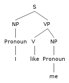
Pronouns (Switchboard corpus [spoken, telephone], Francis et al. 1999)

Pronoun Non-Pronoun

Subject 91% 9 %

Object 34% 66%

Lexical

Left tree is correct for this example
Right tree is correct for

Conjunction ambiguities can create trees to which a PCFG cant assign distinct probabilities, but intuitively, the trees are quite different in probabilitity:

Notice the two trees employ exactly the same bags of rules, so they must, acording to a PCFG, be equiprobable.

Using
grandparents

Johnson (1998) demonstrates the utility of using the grandparent node as a contextual parameter of a probabilistic parsing model.
This option uses more derivational history.

NP₁: P(... | P = NP, GP = S)
NP₂: P(... | P = NP, GP = VP)

Significant improvement on PCFG:

Can capture distributional differences between subject and object NPs (such as likelihood of pronoun)
Outperforms left-corner parser described in Manning and Carpenter (1997)

S → NP VP S → NP^S VP^S

NP → PRP NP^S → PRP

NP^VP → PRP

NP → DT NN NP^S → DT NN

NP^VP → DT NN

This strategy is called splitting. We split the category NP in two so as to model distinct internal distributions depending on the external context of an NP Note that in the work above, preterminals are not split.

Splitting preterminals
Johnson's grandparent grammars work because they reclaim some of the ground lost due to the incorrectness of the independence assumptions of PCFGs. But the other problem for PCFGs that we noted is that they miss lexical dependencies. If we extend the idea of gradparent information to preterminals, we can begin to capture some of that information.

The parse on the left is incorrect because of an incorrect choice between the following two rules:
PP → IN PP
PP → IN SBAR

The parse on the right, in which the categories (including preterminal categories) are annotated with grandparent information, is correct.
The choice is made possible because the string advertising works can be analyzed either as an SBAR or an NP:
[_SBAR Advertising works] when it is clever.
[_NP The advertising works of Andy Warhol] made him a legend.
Now as it happens words of preterminal category IN differ greatly in how likely they are to occur with sentences:

IN SBAR

if John comes

before John comes

after John comes

? under John comes

? behind John comes

So this is a clear case where distributional facts about words helps. And the simple act of extending the grandparent strategy to preterminals helps capture the differences between these two classes of IN.

Generalized
Splitting
Obviously there are many cases where splitting helps.
But there are also cases where splitting hurts. We already have a sparseness problem. If a split results in a defective or under-represented distribution, it can lead to overfitting and it can hurt. Generalizations that were there before the split can be blurred or lost.

Two approaches:
Hand-tuned rules (Klein and Manning 2003b)
Split-and-merge algorithm: search for optimal splits (Petrov et al. 2006)

Lexicalized
CFGs
An extreme form of splitting:

VP → VBD NP PP VP(dumped,VBD) → VBD(dumped,VBD) NP(sacks,NNS) PP(into,P)

VP(sold,VBD) → VBD(sold,VBD) NP(pictures,NNS) PP(of,P)

. . .

Notice categories are being annotated with two kinds of information:

Head word
Category of their immediately dominated head constituent

Lexical rules all have probability 1.0

Sparseness
problems
Maximum likelihood estimates for the PCFG defined by lexicalized splitting are doomed by sparseness: The rule prob for:

VP(dumped,VBD) → VBD(dumped,VBD) NP(sacks,NNS) PP(into,P)

is:

Count(VP(dumped,VBD) → VBD(dumped,VBD) NP(sacks,NNS) PP(into,P))

-----------------------------------------------------------

Count(VP(dumped,VBD))

No corpus is likely to supply reliable counts for such events.
How do we usually solve sparseness problems? We need to make some further independence assumptions!

Collins I
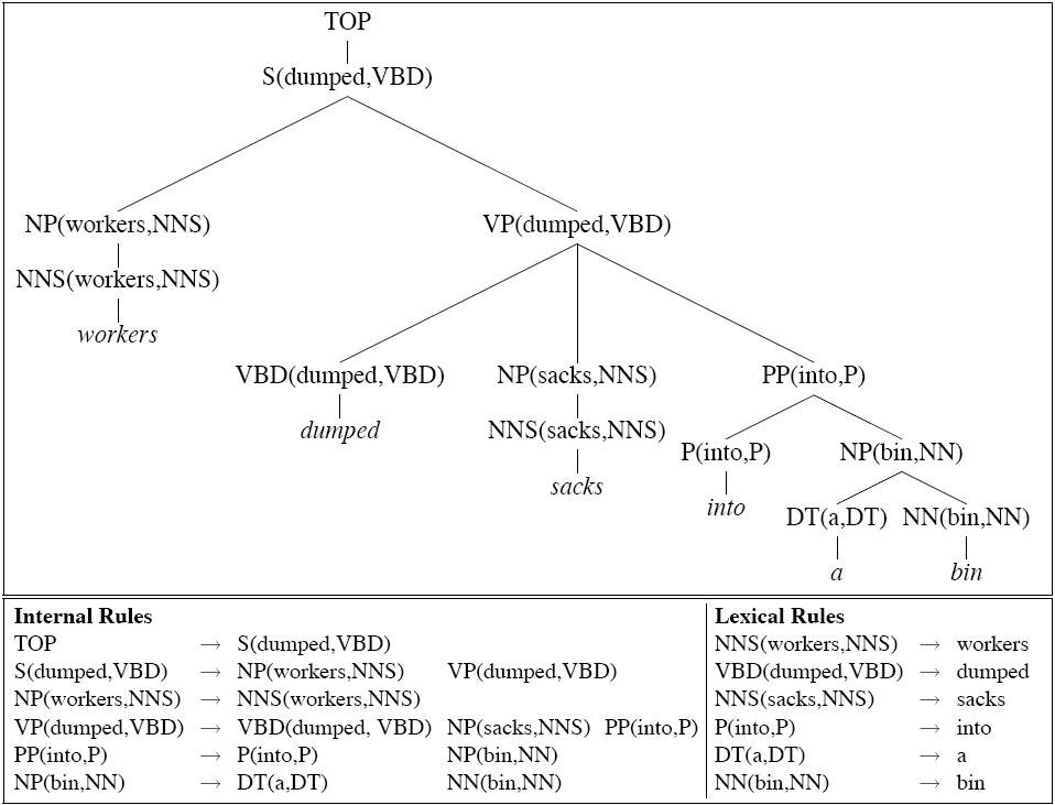
Generation story: Break down a rule into number of contextually dependent subevents which collectively "generate" an occurrence of a rule:
LHS → L_n L_n-1 ... H R₁ .... R_n-1 R_n

Basic decomposition: Generate head first, then L_i modifers terminating with STOP, then R_i modifiers terminating with STOP. For the tree above we have the following sub event probs

P(H|LHS) = P(VBD(dumped,VBD) | VP(dumped,VBD))
P_l(STOP | VP(dumped,VBD), VBD(dumped,VBD))
P_r(NP(sacks,NNS) | VP(dumped,VBD),VBD(dumped,VBD))
note independent of any left modifiers
P_r(PP(into,P) | VP(dumped,VBD),VBD(dumped,VBD)):
note independent of NP(sacks,NNS)
P_r(STOP | VP(dumped,VBD), VBD(dumped,VBD),PP)
Let
R = VP(dumped,VBD) → VBD(dumped,VBD) NP(sacks,NNS) PP(into,P))
We estimate the probability of R by multiplying these probs together:
P(R) =
P(VBD(dumped,VBD) | VP(dumped,VBD)) × P_l(STOP | VP(dumped,VBD), VBD(dumped,VBD)) × P_r(NP(sacks,NNS) | VP(dumped,VBD),VBD(dumped,VBD)) ×
P_r(PP(into,P) | VP(dumped,VBD),VBD(dumped,VBD)) × P_r(STOP | VP(dumped,VBD), VBD(dumped,VBD),PP)

Distance
Collins discovered that adding distance of modifier from head (measured as number of intervening words) is a useful measure:

P(R₂(rh₂,rt₂) | P,H,hw,ht,distance(R₁))

Collins
Backoff

Backoff Level P_R(R_i(rw_i,rt_i |...)) Example

1 P_R(R_i(rw_i,rt_i | P,hw,ht)) P_R(NP(sacks, NNS | VP,VBD,dumped))

2 P_R(R_i(rw_i,rt_i | P, ht)) P_R(NP(sacks, NNS | VP,VBD))

3 P_R(R_i(rw_i,rt_i | P)) P_R(NP(sacks, NNS | VP))

The three models are linearly interpolated.

State of the art
Using the PARSEVAL metric for comparing gold standard and system parse trees (Black et al. 1991), state-of-the-art statistical parsers trained on the Wall Stree Journal treebank are performing at about 90% precision 90% recall.