6.5. Pandas Introduction¶

Pandas is Python’s most popular tool set for manipulating data in tabular form (Excel sheets, data tables). This section has two main goals. The first is to introduce the two main pandas data types, DataFrame and Series.

A DataFrame is a table of data. Datasets at all levels of analysis of analysis can be represented as DataFrames.

A DataFrame has values arranged in rows and column, like a 2D numpy array, but differing from it in two important respects:

Columns often contain data of some non-numerical type, especially strings. Distinct columns in the same DataFrame often contain distinct types. In numpy it’s useful to speak of the type of an array; in pandas, it’s more natural to speak of the type of a column.

A DataFrame uses keyword indexing instead of positional indexing.

Despite the change in how indexing works, all the principles that apply to computing with numpy arrays will carry over with minor modifications to computing with pandas DataFrames. This is especially true of Boolean indexing, which will be your fundamental tool for selecting and reshaping data in pandas. Where a DataFrame is like a 2D array, a Series is like a 1D array; both the rows and the columns of pandas DataFrames are Series objects.

The second goal of this section is to introduce you to some of pandas analytical tools, especially cross-tabulation and grouping,

By the end of the module, we will have covered using pandas for all of the following:

Create Data – We learn how to create pandas DataFrames from raw data in files or in Python containers.

Retrieve Existing Data - We will learn how to read in data from the web and other sources.

Analyze Data. We step though some simple analytical tasks with a number of different datasets, using pivot tables, cross-tabulation,. and grouping.

Present Data. We plot some data in graphs, mostly via the very helpful plotting facilities pandas offers, and peek under the hood a bit at the default pandas backend for plotting, matplotlib.

6.5.1. Create Data¶

Let’s start with a toy dataset, then we’ll ramp up.

The data set will consist of 5 baby names and the number of births recorded for a particular year (1880, as it happens).

# The initial set of baby names and birth rates
names = ['Bob','Jessica','Mary','John','Mel','Mel']
gender = ['M','F','F','M','M','F']
births = [968, 155, 77, 578, 973,45]

To merge these two lists together we will use the zip function.

BabyDataSet = list(zip(names,gender,births))
print(BabyDataSet)

[('Bob', 'M', 968), ('Jessica', 'F', 155), ('Mary', 'F', 77), ('John', 'M', 578), ('Mel', 'M', 973), ('Mel', 'F', 45)]

We next create a DataFrame.

df will be a DataFrame object. You can think of this object holding the contents of the BabyDataSet in a format similar to a sql table or an excel spreadsheet. Lets take a look below at the contents inside df.

df = DataFrame(data = BabyDataSet, columns=['Names', 'Gender', 'Births'],index = ['b','c','e','a','d','f'])
df

	Names	Gender	Births
b	Bob	M	968
c	Jessica	F	155
e	Mary	F	77
a	John	M	578
d	Mel	M	973
f	Mel	F	45

This pandas DataFrame consists of 6 rows and 3 columns. The letters along the left edge are the index. The index provides names or handles for the rows. The column names provide handles for the columns.

One way to think of a DataFrame is as something like a numpy 2D array which uses keyword indexing instead of positional indexing. Thus instead of thinking of the item Mary as being in the row indexed by 2 and the column indexed by 0, we think of it as being in the row indexed by e and the column indexed by Names.

6.5.2. Selecting Columns¶

To explore the idea of a DataFrame as a keyword-indexed 2D array, let’s first look at a 1D object in pandas, a single column.

Columns in a pandas DataFrame are indexed by the column name:

names_col = df['Names']
names_col

b        Bob
c    Jessica
e       Mary
a       John
d        Mel
f        Mel
Name: Names, dtype: object

As the output shows, the row handles are part of the column object. so the element Mary can be accessed by handle e.

names_col['e']

'Mary'

So a column is an object like a numpy 1D array, but indexed by handles like b and e.

The data type of a column in pandas is Series.

type(df['Names'])

pandas.core.series.Series

The natural question to ask next is: Are rows also 1D objects in pandas? And the answer is yes.

We demonstrate that next.

6.5.3. Selecting rows¶

The simplest way of selecting a pandas row is via the .loc attribute:

Given a Dataframe and a row handle, df.loc[RowName] returns the row:

e_row = df.loc['e']
e_row

Names     Mary
Gender       F
Births      77
Name: e, dtype: object

As promised, this too is a Series.

type(e_row)

pandas.core.series.Series

Again it comes with handles for its elements. In this case those handles are column names:

e_row['Names']

'Mary'

The .loc method was needed to define e_row because the df[keyword] syntax is reserved for the case where keyword is a column name. Thus

# This produces a KeyError because 'e' is not a column name.
# df['e']

We’ve now seen two different ways to access the same DataFrame element Mary:

df['Names']['e']

'Mary'

Call the syntax in the previous cell – Column handle first, then row handle – native pandas syntax. In this syntax, the DataFrame is like a dictionary whose keys are column handles, the columns are dictionaries whose keys are row handles.

We then introduced .loc.

df.loc['e']['Names']

'Mary'

Call the syntax with .loc[] numpy-like syntax. The idea is that the syntax of .loc[] works like numpy with keyword indexing instead of positional indexing. The numpy analogue of the syntax in the last cell is

a = np.arange(12).reshape((3,4))
print(a)
r,c,val=2,3,11
print(f'{r=}, {c=} {val=}')

print(f'{a[r][c]=: 3d}')

[[ 0  1  2  3]
 [ 4  5  6  7]
 [ 8  9 10 11]]
r=2, c=3 val=11
a[r][c]= 11

The analogy can be pushed much further. Numpy also allows:

a[r,c]

Paralleling that in pandas, using .loc[], we have:

df.loc['e','Names']

'Mary'

Another similarity with numpy when we use .loc is that we can do slicing.

Repeating df:

df

	Names	Births
b	Bob	968
c	Jessica	155
e	Mary	77
a	John	578
d	Mel	973

we take a row slice:

print(df.loc['c':'a'])
type(df.loc['c':'a'])

     Names  Births
c  Jessica     155
e     Mary      77
a     John     578

pandas.core.frame.DataFrame

We get a sub-DataFrame starting up at row c, going up to and including row e.

What’s a little surprising here is that we got 3 rows, where from all our experience with normal Python slices, we would expect 2. This is not a bug; the motivation is that we are not indexing by position, but by the names of elements in the index. When you want to get a slice that goes from row c to row a, all you have to know is those two names; if we had to use the same convention used with slicing by position, we would also have to know the name of the row following a, which isn’t in general preductable.

As with numpy we can also slice along the column-axis.

df.loc[:,'Gender':'Births']

	Gender	Births
b	M	968
c	F	155
e	F	77
a	M	578
d	M	973
f	F	45

We can also do the pandas equivalent equivalent of fancy indexing in numpy: Pass in a sequence or row handles to get a subset of the rows:

df.loc[['b','c','f']]

	Names	Gender	Births
b	Bob	M	968
c	Jessica	F	155
f	Mel	F	45

As with numpy the extra set of square brackets is required.

And of course we can do fancy-indexing with columns as well. The following command creates a new DataFrame omitting the gender column:

df.loc[:,['Names','Births']]

	Names	Births
b	Bob	968
c	Jessica	155
e	Mary	77
a	John	578
d	Mel	973
f	Mel	45

So we have indexing by keyword and two different ways of specifying it, native-Pandas syntax and numpy-like using .loc[]. Does all this mean positional indexing is completely abandoned in pandas?

No, as we will see, it’s possible, and it’s sometimes essential.

6.5.4. Boolean conditions¶

The most comon way of selecting rows is with a Boolean sequence.

For example, we can select the first, second and fifth rows directly as follows.

df[[True,True,False,False,True,False]]

	Names	Gender	Births
b	Bob	M	968
c	Jessica	F	155
d	Mel	M	973

Or we can use a Boolean Series constructed from a Boolean condition on column values.

df[df['Names']=='Mel']

	Names	Gender	Births
d	Mel	M	973
f	Mel	F	45

This can also be written

df.loc[df['Names']=='Mel']

	Names	Gender	Births
d	Mel	M	973
f	Mel	F	45

We illustrate these constructions in the next few examples.

6.5.5. Selecting Rows with Boolean Conditions¶

Overview: The process of selecting rows by values involves two steps 1. We use a Boolean conditions on a column (a 1D pandas Series object) much as we did on numpy 1D arrays. The result is a Boolean Series. 2. We use the Boolean Series as a mask to select a set of rows, just as we did with arrays.

Placing a Boolean condition on a column works just as it did in numpy, The condition is applied elementwise to the elements in the colomn:

print(df['Births'])
print()
print(df['Births'] > 500)

  968
  155
   77
  578
  973
Name: Births, dtype: int64

   True
  False
  False
   True
   True
Name: Births, dtype: bool

The result is also a Series containing Boolean values.

type(df['Births'] > 500)

pandas.core.series.Series

Continuing the analogy with numpy: Just as we could use a 1D Boolean array as Boolean mask to index a numpy 2D array, so we can use a pandas Boolean Series to mask a pandas DataFrame.

df[df['Births'] > 500]

	Names	Gender	Births
b	Bob	M	968
a	John	M	578
d	Mel	M	973

Given df[BS], where BS is a Boolean Series, pandas will always try to align BS’s index with df’s index to do row selection. That means BS must have the same row handles as df; a mismatch raises an IndexingError.

For example, if we try to use only the first 4 rows of the Boolean Series is the last example:

df[(df['Births'] > 500)[:4]]

/var/folders/w9/bx4mylnd27g_kqqgn5hrn2x40000gr/T/ipykernel_4727/2043702469.py:1: UserWarning: Boolean Series key will be reindexed to match DataFrame index.
  df[(df['Births'] > 500)[:4]]

---------------------------------------------------------------------------

IndexingError                             Traceback (most recent call last)

/var/folders/w9/bx4mylnd27g_kqqgn5hrn2x40000gr/T/ipykernel_4727/2043702469.py in <module>
----> 1 df[(df['Births'] > 500)[:4]]

...

IndexingError: Unalignable boolean Series provided as indexer (index of the boolean Series and of the indexed object do not match).

df[BooleanSeries] is a synonym of df.loc[BooleanSeries]. Hence, the expression in the next cell selects he same rows as the row selection in the last example.

df.loc[df['Births'] > 500]

	Names	Gender	Births
b	Bob	M	968
a	John	M	578
d	Mel	M	973

Notice that this expression has two indexing operations, one with df.loc and one without. The inner one uses what we’ve been calling native pandas like syntax, with a column specification in the square brackets.

It’s possible to write this entirely in numpy-like syntax, but it gets awkward. You would have to use exactly as many :s and ,s as you do in selecting numpy rows:

df.loc[df.loc[:,'Births'] > 500]

	Names	Gender	Births
b	Bob	M	968
a	John	M	578
d	Mel	M	973

This awkwardness is merely a consequence of having the .loc[] syntax work like numpy: in each case, it has to be made clear whether rows or columns are being selected.

That fussiness brings with it some flexibility. We saw above that the .loc[] operator can be used to select columns with fancy-indexing. It can also select them with a Boolean condition. To omit the Gender column, we can do:

df.loc[:,[True,False,True]]

	Names	Births
b	Bob	968
c	Jessica	155
e	Mary	77
a	John	578
d	Mel	973
f	Mel	45

Or we can construct a Boolean Series containing the same Booleans using a condition on columns:

df.loc['a']!='M'

Names      True
Gender    False
Births     True
Name: a, dtype: bool

What columns meet the condition that they don’t have the value M in the a-row? The Names and Births columns. The Gender column, on the other hand does have value M in the a-row, so its Boolean value under this condition is False.

And using this condition as a column-selector, we again construct a DataFrame lacking the gender column.

df.loc[:,df.loc['a']!='M']

	Names	Births
b	Bob	968
c	Jessica	155
e	Mary	77
a	John	578
d	Mel	973
f	Mel	45

As this example suggests, using Boolean conditions to select columns is less useful than using them to select rows. One can imagine situations where a Boolean condition might be the best way to select a set of columns, but they’re not all that common.

Since we will almost always be selecting rows with Boolean conditions we can dispense with using the .loc[] syntax for Boolean conditions. So rather than write:

df.loc[df.loc[:,'Births'] > 500]

	Names	Gender	Births
b	Bob	M	968
a	John	M	578
d	Mel	M	973

we write

df[df['Births'] > 500]

	Names	Gender	Births
b	Bob	M	968
a	John	M	578
d	Mel	M	973

or

df.loc[df['Births'] > 500]

	Names	Gender	Births
b	Bob	M	968
a	John	M	578
d	Mel	M	973

Finally some comments on Boolean coditions and types. We note that Boolean conditions on rows will always return a set of rows, which is always a DataFrame.

Returning to our original example:

mel_rows = df[df['Names']=='Mel']
print(mel_rows)
print(type(mel_rows))

  Names Gender  Births
d   Mel      M     973
f   Mel      F      45
<class 'pandas.core.frame.DataFrame'>

We see that this Boolean condition happens to return a DataFrame with two rows.

If the name is Mary there will just be one row, but what’s returned will still be a DataFrame.

mary_rows = df[df['Names']=='Mary']
print(mary_rows)
print(type(mary_rows))

  Names Gender  Births
e  Mary      F      77
<class 'pandas.core.frame.DataFrame'>

Hence to get to, say, the numerical value for the number of babies with the name Mary, we still need to select along two axes:

df[df['Names']=='Mary']['Births']['e']

6.5.6. Combining Conditions with Boolean operators¶

In numpy & is an operator that performs an elementwise and on two Boolean arrays, producing a Boolean array that only has True wherever both the input arrays have True.

import numpy as np
a = np.array([True,False,True])
b= np.array([False,True,True])
print('a', a)
print('b', b)
print('a & b', a&b)

a [ True False  True]
b [False  True  True]
a & b [False False  True]

Let B1 and B2 be two Boolean Series.

The & operator can also be used to combine two Boolean Series instances. The result is a single Boolean Series that finds the rows that satisfy both conditions.

df

	Names	Births
0	Bob	968
1	Jessica	155
2	Mary	77
3	John	578
4	Mel	973

df[(df['Births'] > 500) & (df['Births'] < 900)]

	Names	Gender	Births
a	John	M	578

Note that the parentheses are needed here.

As with numpy arrays, Series may also be combined with “bitwise not” (~) and “bitwise or” (|).

The names which were used over 500 times but not 578 times:

df[(df['Births'] > 500) & ~(df['Births'] == 578)]

	Names	Gender	Births
b	Bob	M	968
d	Mel	M	973

Applying the condition that the value in the Births column does not fall between 500 and 900, we exclude the "John" row.

df[(df['Births'] < 500) | (df['Births'] > 900)]

	Names	Gender	Births
b	Bob	M	968
c	Jessica	F	155
e	Mary	F	77
d	Mel	M	973
f	Mel	F	45

6.5.7. Keyword indexing and Alignment¶

We have been at pains to emphasize that DataFrames are like 2D arrays but with keyword indexing instead of position based indexing.

One of the consequences of this is that shape is not the decisive factor in determining when two dataFrames can be combined by an operation.

When two numpy arrays of incompatible shapes are combined, the result is an error:

A = np.ones((2,2))
B = np.zeros((3,3))
# This is a Value Error
A + B

---------------------------------------------------------------------------

ValueError                                Traceback (most recent call last)

/var/folders/w9/bx4mylnd27g_kqqgn5hrn2x40000gr/T/ipykernel_76047/1019460503.py in <module>
      2 B = np.zeros((3,3))
      3 # This is a Value Error
----> 4 A + B


ValueError: operands could not be broadcast together with shapes (2,2) (3,3)

We use an example of Jake Van der Plas’s to show the same is not true of pandas DataFrames:

M = np.random.randint(0, 20, (2, 2))
A = pd.DataFrame(M,
                 columns=list('AB'))
A

	A	B
0	11	19
1	18	2

DataFrame A is 2x2.

M = np.random.randint(0, 10, (3, 3))
B = pd.DataFrame(M,
                 columns=list('ABC'))
B

	A	B	C
0	5	3	2
1	6	1	0
2	6	3	7

DataFrame B is 3x3.

Now we combine these seemingly incompatible matrices, A and B:

A+B

	A	B	C
0	16.0	22.0	NaN
1	24.0	3.0	NaN
2	NaN	NaN	NaN

Whereever one of the DataFrames was undefined for a column/row name, we got a NaN. More importantly, wherever we had positions that were defined in both DataFrames, we performed addition.

The usefulness of this emerges when we we try to merge data from two different sources, each of which may have gaps. if we have our row and index labeling aligned, we may still be able to partially unify the information.

What applies to operations on numbers applies equally well to operations on strings. Consider df an df2.

df

	Names	Births
0	Bob	968
1	Jessica	155
2	Mary	77
3	John	578
4	Mel	973

df2

	Names	Births
0	Bob	968
3	John	578
4	Mel	973

The two DataFrames share column names and some index names; one column contains numbers, the other strings.

The + operation — call it addition — is defined on both strings and numbers and will apply to any columns that can be aligned; so examine the 0, 3, 4 rows in the output of the next cell. Note that both columns undergo addition in those rows, while the unshared rows are NaN’ed.

df2 + df

	Names	Births
0	BobBob	1936.0
1	NaN	NaN
2	NaN	NaN
3	JohnJohn	1156.0
4	MelMel	1946.0

This kind of behavior follows from being consistent about keyword indexing and from allowing elementwise operations when possible:

df['Names'] + 'x'

      Bobx
  Jessicax
     Maryx
     Johnx
      Melx
Name: Names, dtype: object

6.5.7.1. Vectorized operations with string `Series`¶

It is worth pointing out that pandas also tries to allow the string analogue of vectorized functions (functions that can be applied elementwise to arrays) whenever possible. Typically, this requires invoking a “StringMethod” accessor on the Series instance.

For example, although df['Names'].lower() is an error, we can acomplish what we’re after here, lowercasing every element in the column, by first calling the .str method, then .lower().

The .str() method provides an accessor to string methods which will apply elementwise:

df['Names'].str

<pandas.core.strings.accessor.StringMethods at 0x7ff488e432e8>

df['Names'].str.lower()

      bob
  jessica
     mary
     john
      mel
Name: Names, dtype: object

We can also use Boolean conditions on strings elementwise to select rows:

df[df['Names'].str.startswith('M')]

	Names	Births
2	Mary	77
4	Mel	973

The following expression returns a Series of first elements, preserving the original indexing.

df['Names'].str[0]

  B
  J
  M
  J
  M
Name: Names, dtype: object

NaNs will as usual give rise to more NaNs, so .str methods will be robust to data gaps.

(df + df2)['Names'].str[0]

    B
  NaN
  NaN
    J
    M
Name: Names, dtype: object

So if we want to collect data on correlations between name gender and name first letters, we can do:

df['Gender'].unique()

array(['M', 'F'], dtype=object)

for g in df['Gender'].unique():
    print(g)
    print(df[df['Gender']==g]['Names'].str[0])
    print()

M
b    B
a    J
d    M
Name: Names, dtype: object

F
c    J
e    M
f    M
Name: Names, dtype: object

6.5.8. Sorting and positional indexing¶

To find the most popular name or the baby name with the highest birth rate, we can do one of the following.

Sort the dataframe and select the top row
Use the max() attribute to find the maximum value

We illustrate these in turn.

Next we create a new DataFrame, sorting the rows according to values in a particular column. This column is called by by argument of the .sort_values() method.

# Method 1 (old pandas)
Sorted_df = df.sort_values('Births', ascending= False)
Sorted_df

	Names	Gender	Births
d	Mel	M	973
b	Bob	M	968
a	John	M	578
c	Jessica	F	155
e	Mary	F	77
f	Mel	F	45

Often we want to be able to find the highest ranked row of such witout knowing its handle, so we are in a situation where keyword-indexing is not what we want.

To get to the actual name that is the most popular one, we need positional indexing (first row after the sort). Fortunately, pandas orovides positional indexing with .iloc[], which has a syntax very similar to .loc[].

Sorted_df.iloc[0]['Names']

'Mel'

Of course if all we were interested in was the count of the most popular name, we could do:

# Method 2:
df['Births'].max()

Note that although we can just as easily sort a column (Series) as a DataFrame, it will be more work to find the associated value in another column.

Illustrating:

print(df['Births'])
SortedBirths = df['Births'].sort_values(ascending=False)
print(SortedBirths)

  968
  155
   77
  578
  973
Name: Births, dtype: int64
  973
  968
  578
  155
   77
Name: Births, dtype: int64

Now to get the most popular name, we must retrieve the first element in the sorted index, and then we can use that index element to get the name:

print(SortedBirths.index[0])
df.loc[SortedBirths.index[0],'Names']

'Mel'

6.5.9. Loading Data: A more realistic example¶

The next cell loads data from my website and will take some time to
execute.
It is slow because it is retrieving a number of large uncompressed
files.
Each file represents a different year of comma-separated (hence .csv
format) babynames data. For example, the start of yob1881.txt
looks like this:

Mary,F,7065
Anna,F,2604
Emma,F,2003
Elizabeth,F,1939
Minnie,F,1746

The code cell below will build a names DataFrame similar to that of our toy example, but much larger and with two new columns, "sex" and "year".

import pandas as pd
years = list(range(1880,2011))
pieces = []
columns = ['name','sex','births']

url = 'https://raw.githubusercontent.com/gawron/'\
       'python-for-social-science/master/pandas/names/'
for year in years:
    path = f'{url}yob{year:d}.txt'
    frame = pd.read_csv(path,names=columns)
    frame['year'] = year
    pieces.append(frame)

names = pd.concat(pieces, ignore_index=True)

We first build the list pieces in the for-loop; pieces is a list of DataFrames. As we process each data file, we keep track of the year by adding a 'year' column to the DataFrame. We then concatenate that list into a single large frame called names, ignoring the indexes in the old frames. We ignore the indexes because they will all be number ranges starting with 0, and rather than have a large number of rows indexed 1 (1 from each year), we renumber them all.

Think about why it’s hard to build the list pieces with a list comprehension instead of the way it’s done in the above cell. Notice the following doesn’t work. Python requires an expression as the first component of a list comprehension. One reason for this is that list comprehensions are supposed to improve readability. Complex sequences of commands don’t do that, and the for-loop above is much more understandable.

pieces = [f=pd.read_csv('names/yob{0:d}.txt'.format(year),names=columns);
          f['year']=year; f
          for year in years]

If you were successful the next cell should evaluate to True. Please re-evaluate the next cell to check.

len(names)  == 1_690_784

True

We now have a large DataFrame of approximately 1.7 million rows, with a default (numerical) index:

names

	name	sex	births	year
0	Mary	F	7065	1880
1	Anna	F	2604	1880
2	Emma	F	2003	1880
3	Elizabeth	F	1939	1880
4	Minnie	F	1746	1880
...	...	...	...	...
1690779	Zymaire	M	5	2010
1690780	Zyonne	M	5	2010
1690781	Zyquarius	M	5	2010
1690782	Zyran	M	5	2010
1690783	Zzyzx	M	5	2010

1690784 rows × 4 columns

The new DataFrame has 1,690,784 rows and 4 columns.

names.info()

<class 'pandas.core.frame.DataFrame'>
RangeIndex: 1690784 entries, 0 to 1690783
Data columns (total 4 columns):
 #   Column  Non-Null Count    Dtype
---  ------  --------------    -----
 0   name    1690784 non-null  object
 1   sex     1690784 non-null  object
 2   births  1690784 non-null  int64
 3   year    1690784 non-null  int64
dtypes: int64(2), object(2)
memory usage: 51.6+ MB

6.5.10. Selection: Selecting parts of Pandas data frames¶

Having created a much larger Pandas DataFrame with babynames data, we return to selecting data.

names1881 = names[names['year'] == 1881]

names1881

	name	sex	births	year
2000	Mary	F	6919	1881
2001	Anna	F	2698	1881
2002	Emma	F	2034	1881
2003	Elizabeth	F	1852	1881
2004	Margaret	F	1658	1881
...	...	...	...	...
3930	Wiliam	M	5	1881
3931	Wilton	M	5	1881
3932	Wing	M	5	1881
3933	Wood	M	5	1881
3934	Wright	M	5	1881

1935 rows × 4 columns

The first ten rows.

print(type(names1881[:10]))
names1881[:10]

<class 'pandas.core.frame.DataFrame'>

	name	sex	births	year
2000	Mary	F	6919	1881
2001	Anna	F	2698	1881
2002	Emma	F	2034	1881
2003	Elizabeth	F	1852	1881
2004	Margaret	F	1658	1881
2005	Minnie	F	1653	1881
2006	Ida	F	1439	1881
2007	Annie	F	1326	1881
2008	Bertha	F	1324	1881
2009	Alice	F	1308	1881

Note that index starts with 2000 because we have retrieved a subset of the rows in the names data, preserving the indexing.

Retrieve the gender column, and display the last part.

names1881['sex'].tail()

  M
  M
  M
  M
  M
Name: sex, dtype: object

A Boolean test, returning a DataFrame that has one column, a column of Booleans.

This shows the 1881 names are gender sorted, with the female names occupying approximately the last half of the data.

print(type(names1881['sex']=='F'))
names1881['sex']=='F'

<class 'pandas.core.series.Series'>

   True
   True
   True
   True
   True
        ...
  False
  False
  False
  False
  False
Name: sex, Length: 1935, dtype: bool

Using the analogue of fancy-indexing in numpy arrays (a list of indices selects a list of rows), you can pick out a subdata frame with a subset of columns, using a list of column names:

print(type(names1881[['sex','births']]))
names1881[['sex','births']]

<class 'pandas.core.frame.DataFrame'>

	sex	births
2000	F	6919
2001	F	2698
2002	F	2034
2003	F	1852
2004	F	1658
...	...	...
3930	M	5
3931	M	5
3932	M	5
3933	M	5
3934	M	5

1935 rows × 2 columns

The indexing conventions we observed in the toy example work here.

indexing a series with a valid index member yields the value at that position in the series:

names1881['sex'][2000]

'F'

That’s why a Series is referred to as an ordered set in the Pandas documentation. There are usually no duplicate names, as with dictionary keys, but there is also ordering.

We can do Boolean selection as with the toy example.

print(type(names1881['name']=='Lee'))
lee_rows = names1881[names1881['name']=='Lee']
print(type(lee_rows))
lee_rows

<class 'pandas.core.series.Series'>
<class 'pandas.core.frame.DataFrame'>

	name	sex	births	year
2258	Lee	F	39	1881
2981	Lee	M	342	1881

So lee_rows is a DataFrame containing only the rows for people named “Lee”.

This example also shows why we shouldn’t use the name column to index the data. There are names that occur in two rows, because they are both male and female names.

You can also pick out a sub data frame with just the female names. We do that and query the “sex” column to show we’ve got a female_rows DataFrame with about half the data of the original DataFrame.

print(type(names1881['sex']=='F'))
female_rows1881 = names1881[names1881['sex']=='F']
print(type(female_rows1881))
female_rows1881.tail()

<class 'pandas.core.series.Series'>
<class 'pandas.core.frame.DataFrame'>

	name	sex	births	year
2933	Tinie	F	5	1881
2934	Tiny	F	5	1881
2935	Vernon	F	5	1881
2936	Verona	F	5	1881
2937	Viney	F	5	1881

Since there are no male rows in female_rows1881, this is an empty DataFrame:

female_rows1881[female_rows1881['sex'] == 'M']

	name	sex	births

len(female_rows1881)

len(names1881)

6.5.11. Summary/Review: Selection & Indexing¶

# Example df for the summary below, lower-case for the index, upper-case for the col names
import pandas as pd
df = pd.DataFrame.from_dict(dict(a=[1,11,111],
                                 b=[2,22,222],
                                 c=[3,33,333],
                                 aa=[1,11,111],
                                 bb=[2,22,222],
                                 cc=[3,33,333]),
                                 orient='index',  # the keyword labeled items are rows
                                 columns=['A',"B","C"]  # need to label the columns independently
                           )
df

	A	B	C
a	1	11	111
b	2	22	222
c	3	33	333
aa	1	11	111
bb	2	22	222
cc	3	33	333

Reviewing and summarizing the discussion above using this example

Selection	Native Pandas	Numpy-like
row	NA	df.loc[‘c’]
row slice	NA	df.loc[‘c’: ‘bb’]
col	df[‘A’]	df.loc[:,‘A’]
row, col	df[‘A’][‘c’]	df.loc[‘c’,‘A’]
		df.loc[‘c’][‘A’]
bool series	df[‘A’] == 2	Not used
bool selection	df[df[‘A’] == 2]	df.loc[df[‘A’] == 2]
row (position)	NA	df.iloc[2]
col (position)	NA	df.iloc[:,2]
fancy (cols)	df[[‘A’,‘C’]]	df.loc[:,[‘A’,‘C’]]
fancy (rows)	NA	df.loc[[‘b’,‘bb’]]

The following cell gives the results of all the selection expressions listed above:

print("\nDataFrame")
print(df)
print("\nrow selection numpylike df.loc['c']")
print(df.loc['c'])
print("\nrow slice numpylike df.loc['c': 'bb']")
print(df.loc['c': 'bb'])
print("\nrow col native pandas df['A']['c']")
print(df['A']['c'])
print("\nrow col numpylike df.loc['c']['A']")
print(df.loc['c']['A'])
print("\nbool series native pandas df['A'] == 2")
print(df['A'] == 2)
print("\nbool selection native pandas df[df['A'] == 2]")
print(df[df['A'] == 2])
print("\nbool selection numpy like df.loc[df['A'] == 2]")
print(df.loc[df['A'] == 2])
print("\nrow (position) df.iloc[2]")
print(df.iloc[2] )
print("\ncol (position) df.iloc[:,2]")
print(df.iloc[:,2])
print("\n fancy indxing cols native pandas df[['A','C']]")
print(df[['A','C']])
print("\n fancy indxing cols numpylike df.loc[:,['A','C']]")
print(df.loc[:,['A','C']])
print("\n fancy indxing row df.loc[['b','bb']")
print(df.loc[['b','bb']])

DataFrame
    A   B    C
a   1  11  111
b   2  22  222
c   3  33  333
aa  1  11  111
bb  2  22  222
cc  3  33  333

row selection numpylike df.loc['c']
A      3
B     33
C    333
Name: c, dtype: int64

row slice numpylike df.loc['c': 'bb']
    A   B    C
c   3  33  333
aa  1  11  111
bb  2  22  222

row col native pandas df['A']['c']
3

row col numpylike df.loc['c']['A']
3

bool series native pandas df['A'] == 2
a     False
b      True
c     False
aa    False
bb     True
cc    False
Name: A, dtype: bool

bool selection native pandas df[df['A'] == 2]
    A   B    C
b   2  22  222
bb  2  22  222

bool selection numpy like df.loc[df['A'] == 2]
    A   B    C
b   2  22  222
bb  2  22  222

row (position) df.iloc[2]
A      3
B     33
C    333
Name: c, dtype: int64

col (position) df.iloc[:,2]
a     111
b     222
c     333
aa    111
bb    222
cc    333
Name: C, dtype: int64

 fancy indxing cols native pandas df[['A','C']]
    A    C
a   1  111
b   2  222
c   3  333
aa  1  111
bb  2  222
cc  3  333

 fancy indxing cols numpylike df.loc[:,['A','C']]
    A    C
a   1  111
b   2  222
c   3  333
aa  1  111
bb  2  222
cc  3  333

 fancy indxing row df.loc[['b','bb']
    A   B    C
b   2  22  222
bb  2  22  222

6.5.12. The .value_counts( ) method¶

Suppose we want to learn the number of distinct male and female names. The easiest way to get that information is by using the Series method .value_counts(). If called by Series S, this method creates a new Series vc indexed by the distinct values of S: the value for each index element of vc is the count of how many times that index element occurred in S.

names1881 = names[names['year']==1881]

names1881['sex'].value_counts()

M    997
F    938
Name: sex, dtype: int64

The sum of the value counts equals the number of rows in names1881:

names1881['sex'].value_counts().sum()

It turns out Series have a plot method; applying that method to the value_counts Series, we get:

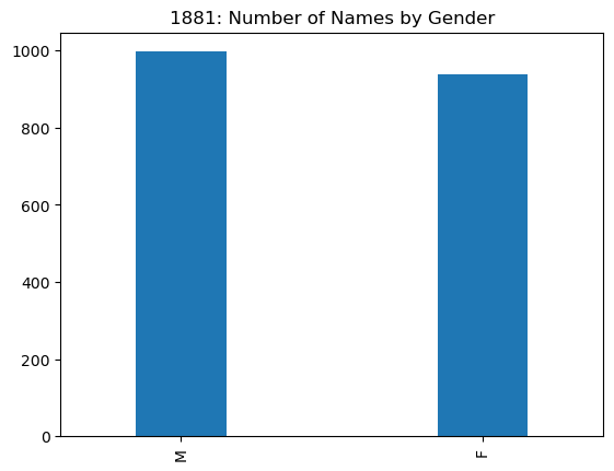
names1881['sex'].value_counts().plot(kind='bar',
                                     width=.3,
                                     title='1881: Number of Names by Gender')

<AxesSubplot:title={'center':'1881: Number of Names by Gender'}>

This is our first very simple example of analytical strategy we will use often with pandas:

Use one of pandas analytical tools to transform the data into a new DataFrame or Series.
Exploit the fact that the transformed data has restructured the index and the columns to make a plot summarizing our analysis.

The plot above shows there were fewer female names than male names in 1881. In fact,

female_names1881 = names1881[names1881['sex']=='F']
len(female_names1881)/len(names1881)

0.4847545219638243

only about 48.5% of the names in use were female.

Translating this code to the entire names data set (1881-2010), we see an interesting change.

print(type(names['sex']=='F'))
female_names = names[names['sex']=='F']
len(female_names)/len(names)

<class 'pandas.core.series.Series'>

0.5937984982114806

names['sex'].value_counts().plot(kind='bar',width=.3,
                                 title='1881--2007: Number of Names by Gender')

<AxesSubplot:title={'center':'1881--2007: Number of Names by Gender'}>

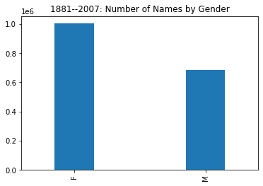
We see the female rows occupy nearly 60% of the data, meaning that some time after 1881 the diversity of female names overtook and greatly surpassed that of male names.

6.5.13. Cross-tabulation¶

To introduce cross-tabulation we will explore the fact we just discovered, that the proportion of female names increases over time

Before doing that, let’s try a simple exercise. If you already know how to do cross-tabulation in pandas, feel free to use it. If you don’t know how to do cross-tabulation in pandas, or perhaps what cross-tabulation is, you should be able to do the problem using your general knowledge of Python.

Plot the proportion of all names that were female names year by year to trace the year by year change.

Hint: create a sequence containing the numbers you need (proportion of female names in each year). Then create a pandas DataFrame female_names_by_year indexed by years with one column (‘Proportion Female Names’). Then do

female_names_by_year.plot()

Note that for this exercise a line connecting the proportion values for each year, which is the default plot type (kind = “line”), is a better choice than a bar plot (kind = “bar”).

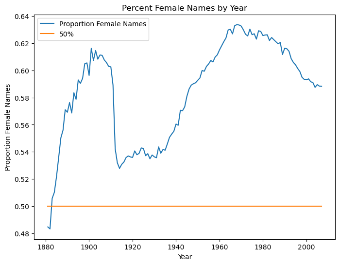
Optionally: Draw a horizontal line at 50% to help the viewer see where the number of female names is greater than that of male names. The births by year plotting example with matplotlib below may help, since this involves some knowledge of matplotlib.

Two answers are provided several cells below.

They are not the only possible answers.

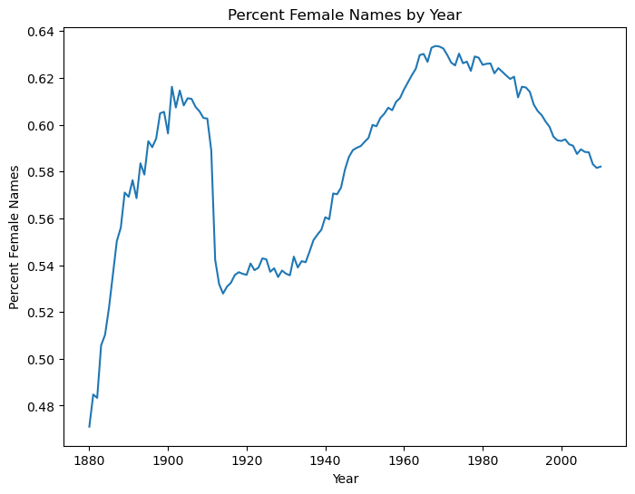
The answer is surprising. Female name diversity is not as simple as a continuously rising trend.

6.5.14. Solution 1¶

The following code is correct, and quite reasonable given what we’ve learned so far in this notebook but unnecessarily complicated. We show a simpler solution below which uses cross-tabulation.

Sine pandas provides some very flexible tools for making a DataFrame from a dictionary, we start with a dictionary comprehension that makes a dictionary with the data we want.

female_names = names[names['sex']=='F']
year_range = range(1881,2008)

def get_proportion_female_names(year):
    # Given a year return the proportion female names that year
    return (female_names['year'] == year).sum()/\
                          (names['year'] == year).sum()

# make a dictionary: year -> proportion of femal enames that year
result = {year: get_proportion_female_names(year) for year in year_range}

Making a DataFrame so we can use its plotting method.

# Dictionary to 1-column DF
# keys in dictionary will be used for the df index
female_names_by_year = \
      pd.DataFrame.from_dict(result,
                             orient='index',
                             columns=['Proportion Female Names'])
female_names_by_year.plot()

<AxesSubplot:>

Here’s the DataFrame we used:

female_names_by_year[:5]

	Proportion Female Names
1881	0.484755
1882	0.483310
1883	0.505758
1884	0.510231
1885	0.521796

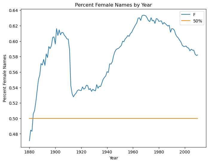
Second plot: Adding The 50% line. Note that we can get two lines just by adding a second column to our female_names_by_year DataFrame.

# Creating axis for plot and secondary line, so a line can be added
from matplotlib import pyplot as plt

# Adding 50% line, using a vectorized assignment to populate
# a new column with a single value.
female_names_by_year['50%'] = .5
# Including axis labels, title
female_names_by_year.plot(xlabel='Year',ylabel='Proportion Female Names',
                           title='Percent Female Names by Year',
                           figsize=(8,6))

<AxesSubplot:title={'center':'Percent Female Names by Year'}, xlabel='Year', ylabel='Proportion Female Names'>

6.5.15. Solution 2¶

A much simpler solution, using the pandas crosstab function:

# This version gives percentages
gender_counts_by_year = pd.crosstab(names['sex'],names['year'],normalize='columns')
gender_counts_by_year

# This version would give us counts rather than percentages
# gender_counts_by_year = pd.crosstab(names['sex'],names['year'])

year	1880	1881	1882	1883	1884	1885	1886	1887	1888	1889	...	2001	2002	2003	2004	2005	2006	2007	2008	2009	2010
sex
F	0.471	0.484755	0.48331	0.505758	0.510231	0.521796	0.535953	0.550358	0.556017	0.571042	...	0.593765	0.591646	0.59104	0.587513	0.589516	0.588384	0.588252	0.583214	0.581556	0.582127
M	0.529	0.515245	0.51669	0.494242	0.489769	0.478204	0.464047	0.449642	0.443983	0.428958	...	0.406235	0.408354	0.40896	0.412487	0.410484	0.411616	0.411748	0.416786	0.418444	0.417873

2 rows × 131 columns

Note that gender_counts_by_year is a DataFrame; the index is the two genders.

It includes percentages (by column) because we passed crosstab the parameter normalize="columns".

This means gender_counts_by_year.loc['F'] is a DataFrame row, that is a Series whose index is the column sequence.

f_row = gender_counts_by_year.loc['F']
f_row

year
  0.471000
  0.484755
  0.483310
  0.505758
  0.510231
          ...
  0.588384
  0.588252
  0.583214
  0.581556
  0.582127
Name: F, Length: 131, dtype: float64

Since a Series has a plot method, we have the following simple option, which leaves out the 50% line.

f_row.plot(ylabel='Percent Female Names',xlabel='Year',
           title='Percent Female Names by Year', figsize=(8,6))

<AxesSubplot:title={'center':'Percent Female Names by Year'}, xlabel='Year', ylabel='Percent Female Names'>

To augment the Solution 2 plot with a 50% line , we can use a DataFrame wrapper containing f_row (as a column) and add a new column for the 50% line.

df2 = pd.DataFrame(f_row)
df2['50%'] = .5
df2.plot(ylabel='Percent Female Names',xlabel='Year',
         title='Percent Female Names by Year', figsize=(8,6))

<AxesSubplot:title={'center':'Percent Female Names by Year'}, xlabel='Year', ylabel='Percent Female Names'>

The lesson of solution 2: If what you’re doing is a pretty standard piece of data analysis, chances are good that pandas includes a simple way of doing it.

Read some documentation to find potential tools. Consult stackoverflow for code snippets and pointers on where to look in the doumentation.

6.5.16. Complaints: a new dataset¶

We’re going to use a new dataset here, to demonstrate how to deal with datasets with few numerical attributes.

The next cell provides a URL for a subset of the of 311 service requests from NYC Open Data.

import os.path
#How to break up long strings into multiline segments
#Note the use of "line continued" character \
data_url = 'https://raw.githubusercontent.com/gawron/python-for-social-science/master/'\
'pandas/datasets/311-service-requests.csv'

import pandas as pd
# Some columns are of mixed types.  This is OK.  But we have to set
# low_memory=False
complaints = pd.read_csv(data_url,low_memory=False)

complaints.info()

<class 'pandas.core.frame.DataFrame'>
RangeIndex: 111069 entries, 0 to 111068
Data columns (total 52 columns):
 #   Column                          Non-Null Count   Dtype
---  ------                          --------------   -----
 Unique Key                      111069 non-null  int64
 Created Date                    111069 non-null  object
 Closed Date                     60270 non-null   object
 Agency                          111069 non-null  object
 Agency Name                     111069 non-null  object
 Complaint Type                  111069 non-null  object
 Descriptor                      110613 non-null  object
 Location Type                   79022 non-null   object
 Incident Zip                    98807 non-null   object
 Incident Address                84441 non-null   object
Street Name                     84432 non-null   object
Cross Street 1                  84728 non-null   object
Cross Street 2                  84005 non-null   object
Intersection Street 1           19364 non-null   object
Intersection Street 2           19366 non-null   object
Address Type                    102247 non-null  object
City                            98854 non-null   object
Landmark                        95 non-null      object
Facility Type                   19104 non-null   object
Status                          111069 non-null  object
Due Date                        39239 non-null   object
Resolution Action Updated Date  96507 non-null   object
Community Board                 111069 non-null  object
Borough                         111069 non-null  object
X Coordinate (State Plane)      98143 non-null   float64
Y Coordinate (State Plane)      98143 non-null   float64
Park Facility Name              111069 non-null  object
Park Borough                    111069 non-null  object
School Name                     111069 non-null  object
School Number                   111048 non-null  object
School Region                   110524 non-null  object
School Code                     110524 non-null  object
School Phone Number             111069 non-null  object
School Address                  111069 non-null  object
School City                     111069 non-null  object
School State                    111069 non-null  object
School Zip                      111069 non-null  object
School Not Found                38984 non-null   object
School or Citywide Complaint    0 non-null       float64
Vehicle Type                    99 non-null      object
Taxi Company Borough            117 non-null     object
Taxi Pick Up Location           1059 non-null    object
Bridge Highway Name             185 non-null     object
Bridge Highway Direction        185 non-null     object
Road Ramp                       180 non-null     object
Bridge Highway Segment          219 non-null     object
Garage Lot Name                 49 non-null      object
Ferry Direction                 24 non-null      object
Ferry Terminal Name             70 non-null      object
Latitude                        98143 non-null   float64
Longitude                       98143 non-null   float64
Location                        98143 non-null   object
dtypes: float64(5), int64(1), object(46)
memory usage: 44.1+ MB

Note that the df.info() summary shows how many non-null values there are in each column, so that you can see there are some columns with very few meaningful entries.

You can see null-entries in the first 5 rows: They are the entries printed out as NaN.

NaN is short for “Not a Number”. It is the standard representation of an undefined result for a numerical calculation. Here it is being used to mean “No data entered here”; NaN is very commonly used with this meaning in pandas, even in columns that do not have a numerical type; we could, alternatively, use Python None for this purpose.

complaints[:5]

	Unique Key	Created Date	Closed Date	Agency	Agency Name	Complaint Type	Descriptor	Location Type	Incident Zip	Incident Address	...	Bridge Highway Name	Bridge Highway Direction	Road Ramp	Bridge Highway Segment	Garage Lot Name	Ferry Direction	Ferry Terminal Name	Latitude	Longitude	Location
0	26589651	10/31/2013 02:08:41 AM	NaN	NYPD	New York City Police Department	Noise - Street/Sidewalk	Loud Talking	Street/Sidewalk	11432	90-03 169 STREET	...	NaN	NaN	NaN	NaN	NaN	NaN	NaN	40.708275	-73.791604	(40.70827532593202, -73.79160395779721)
1	26593698	10/31/2013 02:01:04 AM	NaN	NYPD	New York City Police Department	Illegal Parking	Commercial Overnight Parking	Street/Sidewalk	11378	58 AVENUE	...	NaN	NaN	NaN	NaN	NaN	NaN	NaN	40.721041	-73.909453	(40.721040535628305, -73.90945306791765)
2	26594139	10/31/2013 02:00:24 AM	10/31/2013 02:40:32 AM	NYPD	New York City Police Department	Noise - Commercial	Loud Music/Party	Club/Bar/Restaurant	10032	4060 BROADWAY	...	NaN	NaN	NaN	NaN	NaN	NaN	NaN	40.843330	-73.939144	(40.84332975466513, -73.93914371913482)
3	26595721	10/31/2013 01:56:23 AM	10/31/2013 02:21:48 AM	NYPD	New York City Police Department	Noise - Vehicle	Car/Truck Horn	Street/Sidewalk	10023	WEST 72 STREET	...	NaN	NaN	NaN	NaN	NaN	NaN	NaN	40.778009	-73.980213	(40.7780087446372, -73.98021349023975)
4	26590930	10/31/2013 01:53:44 AM	NaN	DOHMH	Department of Health and Mental Hygiene	Rodent	Condition Attracting Rodents	Vacant Lot	10027	WEST 124 STREET	...	NaN	NaN	NaN	NaN	NaN	NaN	NaN	40.807691	-73.947387	(40.80769092704951, -73.94738703491433)

5 rows × 52 columns

Selecting columns and rows in Complaints

As before we can select a column, by indexing with the name of the column:

complaints['Complaint Type']

0         Noise - Street/Sidewalk
1                 Illegal Parking
2              Noise - Commercial
3                 Noise - Vehicle
4                          Rodent
                   ...
111064    Maintenance or Facility
111065            Illegal Parking
111066    Noise - Street/Sidewalk
111067         Noise - Commercial
111068           Blocked Driveway
Name: Complaint Type, Length: 111069, dtype: object

As above we select rows by constructing Boolean Series:

nypd_bool = (complaints['Agency'] == 'NYPD')
nypd_bool[:10]

   True
   True
   True
   True
  False
   True
   True
   True
   True
   True
Name: Agency, dtype: bool

We construct a sub frame that has only Police Department complaints.

nypd_df = complaints[nypd_bool]

But there are 20 kinds of PD complaints in this data.

complaint_set = nypd_df['Complaint Type'].unique()
complaint_set

array(['Noise - Street/Sidewalk', 'Illegal Parking', 'Noise - Commercial',
       'Noise - Vehicle', 'Blocked Driveway', 'Noise - House of Worship',
       'Homeless Encampment', 'Noise - Park', 'Drinking', 'Panhandling',
       'Derelict Vehicle', 'Bike/Roller/Skate Chronic', 'Animal Abuse',
       'Traffic', 'Vending', 'Graffiti', 'Posting Advertisement',
       'Urinating in Public', 'Disorderly Youth', 'Illegal Fireworks'],
      dtype=object)

So we limit it further:

il_df = nypd_df[nypd_df['Complaint Type'] == 'Illegal Parking']

More constraints means progressively smaller DataFrames:

(len(complaints), len(nypd_df), len(il_df))

(111069, 15295, 3343)

Attribute syntax versus indexing syntax

Note that columns can also be specified using instance/attribute syntax, as in:

complaints.Agency

0          NYPD
1          NYPD
2          NYPD
3          NYPD
4         DOHMH
          ...
111064      DPR
111065     NYPD
111066     NYPD
111067     NYPD
111068     NYPD
Name: Agency, Length: 111069, dtype: object

But also note that doesnt work for the column name Complaint Type; because this has a space, trying to use it as an attribute raises a SyntaxError: No Python name can contain a space; that includes attribute names.

complaints.Complaint Type

  File "/var/folders/_q/2s1hy5bx1l7f9j1lw9zjgt19_wb463/T/ipykernel_64611/2805497044.py", line 1
    complaints.Complaint Type
                            ^
SyntaxError: invalid syntax

So the general Python syntax for indexing a container (square bracket syntax)

complaints['Complaint Type']

is the one to remember.

The indexing syntax is also the one that extends to accommodate selection of multiple columns, using the fancy-indexing convention from numpy (index via an arbitrary sequence of indices).

complaints[['Complaint Type', 'Borough']][:10]

	Complaint Type	Borough
0	Noise - Street/Sidewalk	QUEENS
1	Illegal Parking	QUEENS
2	Noise - Commercial	MANHATTAN
3	Noise - Vehicle	MANHATTAN
4	Rodent	MANHATTAN
5	Noise - Commercial	QUEENS
6	Blocked Driveway	QUEENS
7	Noise - Commercial	QUEENS
8	Noise - Commercial	MANHATTAN
9	Noise - Commercial	BROOKLYN

Narrowing down the set of columns is a common step, especially important when performing further analytical caulculations like pivot tables.

6.5.16.1. Using crosstab with the complaints data¶

The idea of crosstabulation has already arisen. In its simplest form, cross-tabulation is just getting the coocurrence counts of two attributes. In the complaints domain, for example, we might be interested in how often each complaint tyope occurs in each borough.

Crosstab Problem A: For each complaint type, find its frequency in each borough.

This is a cross-tabulation question: We use crosstab to get the joint distribution counts for two attributes.

pd.crosstab(complaints['Agency'],complaints['Borough'])

Borough	BRONX	BROOKLYN	MANHATTAN	QUEENS	STATEN ISLAND	Unspecified
Agency
3-1-1	0	8	11	12	1	60
CHALL	0	0	0	0	0	77
COIB	0	0	0	0	0	1
DCA	155	357	358	284	36	215
DEP	791	2069	3419	1916	690	12
DFTA	4	5	3	3	0	7
DHS	6	31	54	8	0	2
DOB	358	775	477	1257	147	0
DOE	17	26	24	15	7	8
DOF	78	149	215	116	6	5806
DOHMH	657	891	913	602	174	0
DOITT	3	8	15	2	3	0
DOP	0	0	0	0	0	2
DOT	2605	5313	4182	4164	1123	320
DPR	438	1292	407	1934	532	11
DSNY	1094	2966	1167	2579	563	16
EDC	1	23	66	9	0	0
FDNY	6	17	517	52	10	29
HPD	11493	13871	7866	4986	851	0
HRA	0	0	0	0	0	392
NYPD	1933	4886	3657	4154	663	2
OATH	0	0	0	0	0	4
OEM	0	0	0	0	0	29
OMB	0	0	0	0	0	1
OPS	0	0	0	0	0	8
TLC	47	203	937	188	11	105

Elaboration of Crosstab Problem A: For each complaint type, find its frequency in each borough. Also give the total number of complaints by borough and by complaint type.

ct_agency_borough = pd.crosstab(complaints['Agency'],complaints['Borough'],margins=True)
ct_agency_borough

Borough	BRONX	BROOKLYN	MANHATTAN	QUEENS	STATEN ISLAND	Unspecified	All
Agency
3-1-1	0	8	11	12	1	60	92
CHALL	0	0	0	0	0	77	77
COIB	0	0	0	0	0	1	1
DCA	155	357	358	284	36	215	1405
DEP	791	2069	3419	1916	690	12	8897
DFTA	4	5	3	3	0	7	22
DHS	6	31	54	8	0	2	101
DOB	358	775	477	1257	147	0	3014
DOE	17	26	24	15	7	8	97
DOF	78	149	215	116	6	5806	6370
DOHMH	657	891	913	602	174	0	3237
DOITT	3	8	15	2	3	0	31
DOP	0	0	0	0	0	2	2
DOT	2605	5313	4182	4164	1123	320	17707
DPR	438	1292	407	1934	532	11	4614
DSNY	1094	2966	1167	2579	563	16	8385
EDC	1	23	66	9	0	0	99
FDNY	6	17	517	52	10	29	631
HPD	11493	13871	7866	4986	851	0	39067
HRA	0	0	0	0	0	392	392
NYPD	1933	4886	3657	4154	663	2	15295
OATH	0	0	0	0	0	4	4
OEM	0	0	0	0	0	29	29
OMB	0	0	0	0	0	1	1
OPS	0	0	0	0	0	8	8
TLC	47	203	937	188	11	105	1491
All	19686	32890	24288	22281	4817	7107	111069

Now ct_agency_borough contains both an 'All' column (containing the sum of the values in each row) and an 'All' row (containing the sum of the values for each column).

Note that as long as there are no rows missing an 'Agency' or 'Borough' (there aren’t), then ct_agency_borough['All']['All'] is the total number of rows in complaints.

print(len(complaints))
print(ct_agency_borough['All']['All'])

111069
111069

Complaints Problem B: What’s the noisiest borough? A little preprocessing is required. Then we can turn this into a cross tabulation of a restricted set of complaint types and borough.

# Apply a function that returns True if a string starts with 'noise'
# to every element of the Complaint Type column, producing a Boolean Series
# Roughly equivalent to
# boolean_series = pd.Series([ct.startswith('Noise')
#                             for ct in complaints['Complaint Type']])
boolean_series = complaints['Complaint Type'].apply(lambda x: x.startswith('Noise'))
complaints_noise = complaints[boolean_series]
complaints_noise[:5]

	Unique Key	Created Date	Closed Date	Agency	Agency Name	Complaint Type	Descriptor	Location Type	Incident Zip	...
0	26589651	10/31/2013 02:08:41 AM	NaN	NYPD	New York City Police Department	Noise - Street/Sidewalk	Loud Talking	Street/Sidewalk	11432	...
2	26594139	10/31/2013 02:00:24 AM	10/31/2013 02:40:32 AM	NYPD	New York City Police Department	Noise - Commercial	Loud Music/Party	Club/Bar/Restaurant	10032	...
5	26592370	10/31/2013 01:46:52 AM	NaN	NYPD	New York City Police Department	Noise - Commercial	Banging/Pounding	Club/Bar/Restaurant	11372	...

So what’s the noisiest borough? The answer is no surprise to those who’ve been in NYC.

ct_noise = pd.crosstab(complaints_noise['Borough'],complaints_noise['Complaint Type'],
                       margins=True)
ct_noise.sort_values(by = 'All',ascending=False)

Complaint Type	Noise	Noise - Commercial	Noise - Helicopter	Noise - House of Worship	Noise - Park	Noise - Street/Sidewalk	Noise - Vehicle	All
Borough
All	3321	2578	99	67	191	1928	750	8934
MANHATTAN	1848	1140	66	16	91	917	255	4333
BROOKLYN	767	775	23	23	60	456	237	2341
QUEENS	418	451	9	15	27	226	130	1276
BRONX	168	136	1	11	9	292	102	719
STATEN ISLAND	115	76	0	2	4	36	25	258
Unspecified	5	0	0	0	0	1	1	7

Complaints problem C

Find the complaint counts for three agences (‘DOT’, “DOP”, ‘NYPD’).

First Produce a DataFrame containing only the three agencies DT, DOP and NYPD. This part is easy.

pt00 = complaints[complaints.Agency.isin(['DOT', "DOP", 'NYPD'])]

The frame pt00 now restricts us to three agencies.

Second, use pt00 to create a DataFrame or Series whose index is the complaint types and whose three columns are the Three Agencies. Each cell should contain the count of the complaint type of that row and the agency of that column. For example, the number in the 'Animal Abuse' row in the 'NYPD' column should be the number of NYPD complaints about animal abuse (which happens to be 164).

three = ['DOT', "DOP", 'NYPD']
pt00 = complaints[complaints.Agency.isin(three)]
pd.crosstab(pt00['Complaint Type'], pt00['Agency'])

Agency	DOP	DOT	NYPD
Complaint Type
Agency Issues	0	20	0
Animal Abuse	0	0	164
Bike Rack Condition	0	7	0
Bike/Roller/Skate Chronic	0	0	32
Blocked Driveway	0	0	4590
Bridge Condition	0	20	0
Broken Muni Meter	0	2070	0
Bus Stop Shelter Placement	0	14	0
Compliment	0	1	0
Curb Condition	0	66	0
DOT Literature Request	0	123	0
Derelict Vehicle	0	0	803
Disorderly Youth	0	0	26
Drinking	0	0	83
Ferry Complaint	0	4	0
Ferry Inquiry	0	32	0
Ferry Permit	0	1	0
Graffiti	0	0	13
Highway Condition	0	130	0
Highway Sign - Damaged	0	1	0
Homeless Encampment	0	0	269
Illegal Fireworks	0	0	3
Illegal Parking	0	0	3343
Invitation	1	0	0
Municipal Parking Facility	0	1	0
Noise - Commercial	0	0	2578
Noise - House of Worship	0	0	67
Noise - Park	0	0	191
Noise - Street/Sidewalk	0	0	1928
Noise - Vehicle	0	0	750
Panhandling	0	0	23
Parking Card	0	8	0
Posting Advertisement	0	0	5
Public Toilet	0	6	0
Request for Information	1	0	0
Sidewalk Condition	0	339	0
Street Condition	0	3473	0
Street Light Condition	0	7117	0
Street Sign - Damaged	0	691	0
Street Sign - Dangling	0	110	0
Street Sign - Missing	0	327	0
Traffic	0	0	168
Traffic Signal Condition	0	3145	0
Tunnel Condition	0	1	0
Urinating in Public	0	0	30
Vending	0	0	229

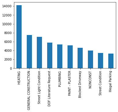
**Crosstab Problem D: What’s the most common complaint type?

Note: This is not a question requiring cross-tabulation. Cross tabulation is for looking at co-occurrence counts of more than one column. This is about sorting the counts of the values occurring in one column, "Complaint Type" For this we use the series method .value_counts() which by default sorts the counts.

complaint_counts = complaints['Complaint Type'].value_counts()
complaint_counts

HEATING                           14200
GENERAL CONSTRUCTION               7471
Street Light Condition             7117
DOF Literature Request             5797
PLUMBING                           5373
                                  ...
Municipal Parking Facility            1
Tunnel Condition                      1
DHS Income Savings Requirement        1
Stalled Sites                         1
X-Ray Machine/Equipment               1
Name: Complaint Type, Length: 165, dtype: int64

Since complaints_counts is a Series (the complaint types are the index) ordered by number of complaints, we can plot the numbers for the top complaint types, demonstrating visually what an outlier Heating is (Oh those NYC winters!).

complaint_counts[:10].plot(kind='bar')

<AxesSubplot:>

Crosstab understanding exercise

Find the distribution of complaint Statuses. That is, write an expression that produces a DataFrame or Series whose index is the seven possible complaint Statuses and whose values are the number of complaints with each Status.

To help you check your solution, here are the seven complaint statuses.

set(complaints['Status'])

{'Assigned',
 'Closed',
 'Email Sent',
 'Open',
 'Pending',
 'Started',
 'Unassigned'}

sc = complaints['Status'].value_counts()
sc

Closed        57165
Open          43972
Assigned       6189
Pending        3165
Started         447
Email Sent      129
Unassigned        2
Name: Status, dtype: int64

6.5.17. Using groupby¶

Grouping is a fundamental data analysis operation. For example, it is the first step in doing a cross-tabulation. We will also see that it us the first step in creating a pivot table.

As these examples suggest, we’re mostly interested in grouping as a preliminary step in performing statistical analysis, but it is useful to look at in isolation first, using the basic groupby function that pandas provides.

Let’s use a new dataset to illustrate, because it has some very natural groupings.

nba_file_url = 'https://gawron.sdsu.edu/python_for_ss/course_core/data/nba.csv'
nba_df = pd.read_csv(nba_file_url)

Each row contains information about one current player. The team rosters are listed in alphabetical order of team name, with the players in alphabetical order by name within the teams.

nba_df[:5]

	Name	Team	Number	Position	Age	Height	Weight	College	Salary
0	Avery Bradley	Boston Celtics	0.0	PG	25.0	6-2	180.0	Texas	7730337.0
1	Jae Crowder	Boston Celtics	99.0	SF	25.0	6-6	235.0	Marquette	6796117.0
2	John Holland	Boston Celtics	30.0	SG	27.0	6-5	205.0	Boston University	NaN
3	R.J. Hunter	Boston Celtics	28.0	SG	22.0	6-5	185.0	Georgia State	1148640.0
4	Jonas Jerebko	Boston Celtics	8.0	PF	29.0	6-10	231.0	NaN	5000000.0

We are going to use it to find out about team salaries, height by position and weight by position.

We group the rows by team and then show the alphabetically first player in each team.

gt = nba_df.groupby('Team')
# First member of each team grouop for first 5 teams
gt.first()[:5]

	Name	Number	Position	Age	Height	Weight	College	Salary
Team
Atlanta Hawks	Kent Bazemore	24.0	SF	26.0	6-5	201.0	Old Dominion	2000000.0
Boston Celtics	Avery Bradley	0.0	PG	25.0	6-2	180.0	Texas	7730337.0
Brooklyn Nets	Bojan Bogdanovic	44.0	SG	27.0	6-8	216.0	Oklahoma State	3425510.0
Charlotte Hornets	Nicolas Batum	5.0	SG	27.0	6-8	200.0	Virginia Commonwealth	13125306.0
Chicago Bulls	Cameron Bairstow	41.0	PF	25.0	6-9	250.0	New Mexico	845059.0

type(gt)

pandas.core.groupby.generic.DataFrameGroupBy

Here we’ve created a DataFrameGroupBy instance that split the player data into subgroups, the players belonging to each team.

We can display one of those groups as follows:

# A particular group
gt.get_group('Utah Jazz')[:5]

	Name	Team	Number	Position	Age	Height	Weight	College	Salary
442	Trevor Booker	Utah Jazz	33.0	PF	28.0	6-8	228.0	Clemson	4775000.0
443	Trey Burke	Utah Jazz	3.0	PG	23.0	6-1	191.0	Michigan	2658240.0
444	Alec Burks	Utah Jazz	10.0	SG	24.0	6-6	214.0	Colorado	9463484.0
445	Dante Exum	Utah Jazz	11.0	PG	20.0	6-6	190.0	NaN	3777720.0
446	Derrick Favors	Utah Jazz	15.0	PF	24.0	6-10	265.0	Georgia Tech	12000000.0

This, however, is an odd use of a grouping object. If all we were interested in was constructing a DataFrame limited to one team, we could accomplished that much more easily with:

nba_df[nba_df['Team'] == 'Utah Jazz'][:5]

	Name	Team	Number	Position	Age	Height	Weight	College	Salary
442	Trevor Booker	Utah Jazz	33.0	PF	28.0	6-8	228.0	Clemson	4775000.0
443	Trey Burke	Utah Jazz	3.0	PG	23.0	6-1	191.0	Michigan	2658240.0
444	Alec Burks	Utah Jazz	10.0	SG	24.0	6-6	214.0	Colorado	9463484.0
445	Dante Exum	Utah Jazz	11.0	PG	20.0	6-6	190.0	NaN	3777720.0
446	Derrick Favors	Utah Jazz	15.0	PF	24.0	6-10	265.0	Georgia Tech	12000000.0

The benefit of the grouping object is that it makes various comparisons based on the same grouping easier. Suppose, for example, that we were interested in comparing average team ages and average team salary. To make this more interested, let’s say we’re interested in looking at the degree of correlation team age and team salary.

Then we use our team grouping instance gt to look at both variables:

mean_age_by_team = gt['Age'].mean()
mean_salary_by_team = gt['Salary'].mean()
comp = pd.DataFrame(dict(Age=mean_age_by_team,
                         Salary=mean_salary_by_team))
comp[:5]

	Age	Salary
Team
Atlanta Hawks	28.200000	4.860197e+06
Boston Celtics	24.733333	4.181505e+06
Brooklyn Nets	25.600000	3.501898e+06
Charlotte Hornets	26.133333	5.222728e+06
Chicago Bulls	27.400000	5.785559e+06

And now it’s quite easy to summon up the correlation of Age and Salary viewed team by team.

#Uses pearsonr correlation
comp_corr = comp.corr()
#Add some color coding to highlight the strong correlations.
comp_corr.style.background_gradient(cmap='coolwarm')

	Age	Salary
Age	1.000000	0.716125
Salary	0.716125	1.000000

The DataFrame.corr() method always produces a square NxN DataFrame. When there are more than two columns, all pairwise correlations are computed. When seeking pairwise correlation only between two columns, use Series.corr:

comp['Age'].corr(comp['Salary'], method='kendall')

0.6398163039514194

Notice that in order to run the .corr() method on the DataFrame comp we first had to create comp with the right index and columns. We did that in line 3 in the cell computing the group means:

comp = pd.DataFrame(dict(Age=mean_age_by_team,
                         Salary=mean_salary_by_team))

Creating this DataFrame was step three of a three-step process:

Grouping by team (sometimes called splitting)
1. gt = nba_df.groupby('Team')
Applying a statistical aggregation function (.mean(...))
1. mean_age_by_team = gt['Age'].mean()
2. mean_salary_by_team = gt['Salary'].mean()
Combining the results into a DataFrame
1. pd.DataFrame(dict(Age=mean_age_by_team, Salary=mean_salary_by_team))

These three steps collectively are called the Split/Apply/Combine strategy. They arise often enough in Statistical Data Analysis to deserve packaging into a single function called pivot_table. For example, to get the mean ages and salaries team by team, we do:

# Group the players into teams, take the mean age and salary for each time,
# make a datafra,
pd.pivot_table(nba_df,index='Team', values=["Salary","Age"],aggfunc='mean')[:5]

	Age	Salary
Team
Atlanta Hawks	28.200000	4.860197e+06
Boston Celtics	24.733333	4.181505e+06
Brooklyn Nets	25.600000	3.501898e+06
Charlotte Hornets	26.133333	5.222728e+06
Chicago Bulls	27.400000	5.785559e+06

Ths is exactly the same DataFrame we saw before created in one step.

We’ll have quite a bit more to say about pivot tables in the second pandas notebook. For now let’s continue exploring the uses of grouping.

There are two motivations for pandas to provide users with direct acces to groupby instances.

A single groupby instance can support the analysis of multiple variables, possibly with different aggregation functions (in our salart and age example we used mean twice).
Grouping can also be done using more than one variable.

Let’s illustrate point (2) by grouping by team and position.

In basketball each team puts five players on the court at any given time. Although the specialized roles of the players on the court are changing, classically a player plays one of five positions:

Point Guard (PG)
Shooting Guard (SG)
Small Forward (SF)
Power Forward (PF)
Center (C).

This data set assigns each player to one of these five positions. A team will typically have multiple players assigned to any given position.

gtp = nba_df.groupby(['Team','Position'])
# Show the first entry for each team/position pair
gtp.first()

		Name	Number	Age	Height	Weight	College	Salary
Team	Position
Atlanta Hawks	C	Al Horford	15.0	30.0	6-10	245.0	Florida	12000000.0
	PF	Kris Humphries	43.0	31.0	6-9	235.0	Minnesota	1000000.0
	PG	Dennis Schroder	17.0	22.0	6-1	172.0	Wake Forest	1763400.0
	SF	Kent Bazemore	24.0	26.0	6-5	201.0	Old Dominion	2000000.0
	SG	Tim Hardaway Jr.	10.0	24.0	6-6	205.0	Michigan	1304520.0
...	...	...	...	...	...	...	...	...
Washington Wizards	C	Marcin Gortat	13.0	32.0	6-11	240.0	North Carolina State	11217391.0
	PF	Drew Gooden	90.0	34.0	6-10	250.0	Kansas	3300000.0
	PG	Ramon Sessions	7.0	30.0	6-3	190.0	Nevada	2170465.0
	SF	Jared Dudley	1.0	30.0	6-7	225.0	Boston College	4375000.0
	SG	Alan Anderson	6.0	33.0	6-6	220.0	Michigan State	4000000.0

149 rows × 7 columns

gtp_first is a DataFrame with a double index (an index with two levels) so we can select an index member from the first level to get a set of rows.

The alphabetically first players on the Boston Celtics, by position.

#
gtp.first().loc['Boston Celtics']

	Name	Number	Age	Height	Weight	College	Salary
Position
C	Kelly Olynyk	41.0	25.0	7-0	238.0	Gonzaga	2165160.0
PF	Jonas Jerebko	8.0	29.0	6-10	231.0	LSU	5000000.0
PG	Avery Bradley	0.0	25.0	6-2	180.0	Texas	7730337.0
SF	Jae Crowder	99.0	25.0	6-6	235.0	Marquette	6796117.0
SG	John Holland	30.0	27.0	6-5	205.0	Boston University	1148640.0

gtp.first().loc['Golden State Warriors']

	Name	Number	Age	Height	Weight	College	Salary
Position
C	Andrew Bogut	12.0	31.0	7-0	260.0	Utah	13800000.0
PF	Draymond Green	23.0	26.0	6-7	230.0	Michigan State	14260870.0
PG	Stephen Curry	30.0	28.0	6-3	190.0	Davidson	11370786.0
SF	Harrison Barnes	40.0	24.0	6-8	225.0	North Carolina	3873398.0
SG	Leandro Barbosa	19.0	33.0	6-3	194.0	Belmont	2500000.0

To get to an individual player record (a row) you need to supply an index member from each level.

So the alphabetically first center on the Boston Celtics is:

gtp.first().loc[('Boston Celtics','C')]

Name       Kelly Olynyk
Number             41.0
Age                25.0
Height              7-0
Weight            238.0
College         Gonzaga
Salary        2165160.0
Name: (Boston Celtics, C), dtype: object

Now a DataFrameGroupBy instance is not a DataFrame or a Series, making groupby one of the few commonly used pandas analysis methods that doesn’t return either:

gtp

<pandas.core.groupby.generic.DataFrameGroupBy object at 0x7fd6c3fdfa20>

But one can do many of the things one does to a DataFrame to a GroupByDataFrame instance. For example, extract a column:

gtp['Salary']

<pandas.core.groupby.generic.SeriesGroupBy object at 0x7fd69ca46438>

Which yields a SeriesGroupBy instance. Which has many of the same methods we saw for the DataFrameGroupBy instances above, including .first() and .get_group().

Instead of calling either of those, let’s apply an aggregation function appropriate to this column:

salary_df = gtp['Salary'].mean()

This gets us a new Series, doubly indexed by team and position:

type(salary_df)

pandas.core.series.Series

salary_df.iloc[:14]

Team                   Position
Atlanta Hawks          C           7.585417e+06
                       PF          5.988067e+06
                       PG          4.881700e+06
                       SF          3.000000e+06
                       SG          2.607758e+06
Boston Celtics         C           2.450465e+06
                       PF          6.056987e+06
                       PG          4.974652e+06
                       SF          6.796117e+06
                       SG          2.107997e+06
Brooklyn Nets          C           1.031814e+07
                       PF          3.576205e+06
                       PG          2.915759e+06
                       SG          1.473351e+06
Name: Salary, dtype: float64

salary_df.loc['Boston Celtics']

Position
C     2.450465e+06
PF    6.056987e+06
PG    4.974652e+06
SF    6.796117e+06
SG    2.107997e+06
Name: Salary, dtype: float64

salary_df.loc['Boston Celtics']['C']

2450465.0

Sample Interpretation: The Celtics pays their centers an average of 2.4 Million.

Now we can do things like the following.

Compare Golden State salaries with Boston salaries position by position.

salary_df.loc['Boston Celtics']

Position
C     2.450465e+06
PF    6.056987e+06
PG    4.974652e+06
SF    6.796117e+06
SG    2.107997e+06
Name: Salary, dtype: float64

salary_df.loc['Golden State Warriors']

Position
C     6.541249e+06
PF    7.275312e+06
PG    8.457256e+06
SF    3.766367e+06
SG    6.316092e+06
Name: Salary, dtype: float64

salary_df.loc['Golden State Warriors'] > salary_df.loc['Boston Celtics']

Position
C      True
PF     True
PG     True
SF    False
SG     True
Name: Salary, dtype: bool

The Warriors pay more at every position but small forward (SF).

Each of these is a Series so in theory we can take the mean again:

salary_df = gtp['Salary'].mean()
print(f'{salary_df.loc["Boston Celtics"].mean():6,.2f}')
print(f'{salary_df.loc["Golden State Warriors"].mean():6,.2f}')
#salary_df.loc['Golden State Warriors'].mean())

4,477,243.37
6,471,255.35

But these numbers may not have the interpretation you think they do.

In order to get the right interpretation of the above numbers, think about why the following numbers aren’t the same.

salary_df2 = gt['Salary'].mean()
print(f'{salary_df2.loc["Boston Celtics"]:6,.2f}')
print(f'{salary_df2.loc["Golden State Warriors"]:6,.2f}')

4,181,504.86
5,924,599.80

6.5.18. Understanding cross-tabulation¶

With the help of the grouping operation we’re now in a position to be able to characterize cross-tabulation a little more generally.

Grouping is the first step in cross-tabulation (which actually uses all three steps of the split/apply/combine strategy).

Let’s take our group-by-team-and-position object and compute the size of each group.

The result is a doubly indexed Series containing group sizes:

#  This with-construction executes code in a CONTEXT
#  which then goes away after the code block is exited.
#  Here we ask pandas to print more than the default number of rows
with pd.option_context('display.max_rows', None):
    print(type(gtp['Name'].count()))
    print(gtp['Name'].count()[:19])

<class 'pandas.core.series.Series'>
Team               Position
Atlanta Hawks      C           3
                   PF          4
                   PG          2
                   SF          2
                   SG          4
Boston Celtics     C           3
                   PF          3
                   PG          4
                   SF          1
                   SG          4
Brooklyn Nets      C           2
                   PF          4
                   PG          3
                   SG          6
Charlotte Hornets  C           3
                   PF          3
                   PG          3
                   SF          1
                   SG          5
Name: Name, dtype: int64

This is exactly the same information we would get with a cross-tabulation, except that the result is packaged in a singly indexed DataFrame with multiple columns:

tp_ct = pd.crosstab(nba_df['Team'], nba_df['Position'],margins=True)
print(type(tp_ct))
tp_ct[:4]

<class 'pandas.core.frame.DataFrame'>

Position	C	PF	PG	SF	SG	All
Team
Atlanta Hawks	3	4	2	2	4	15
Boston Celtics	3	3	4	1	4	15
Brooklyn Nets	2	4	3	0	6	15
Charlotte Hornets	3	3	3	1	5	15
....
All	78	100	92	85	102	457

It is useful to think of cross-tabulation in terms of the split/apply/combine strategy.

Splitting the data into the groups defined by the input sequences.
Applying the operation of counting to the groups.
Combining the results into a DataFrame.

We will return to the split/apply/combine strategy in part two of the pandas introduction.

6.5.19. Exercises combining everything we’ve learned in Part One.¶

Try answering the following questions. Note. You may or may not have to use groupby method in your answers. Even if you know how to use pandas pivot_table function, try to avoid using that. Answers follow a few cells down.

How many NBA players weigh under 220?
By position, how many players weigh under 220? How many do not? In other words, create a DataFrame whose index is position with two columns, False and True, which contain the counts of the players under and not under 220.
What is the average weight of Centers in the league? Which position is heavier on average, Center or Power Forward?
What is the average height of Centers in the league? Which position is taller on average, Center or Power Forward? Note: This is not just a boring minor variation on the previous question. There is a complication.
What position earns the highest salary on average?
What colleges have supplied the most current NBA players? How many colleges have supplied only one NBA player?

#1

#2

#3

#4

#5

#6

#7

Q1 How many NBA players weigh under 220?

len(nba_df[nba_df['Weight']<220])

Q2 By position, how many NBA players weigh under 220?

This is a cross tabulation question; for each position we want the distribution of counts of players over and under 220. The only problem is that we don’t have an over-under 220 column. So we use a Boolean constraint to create one (we don’t need to make it an official column). Then we do a cross-tabulation.

# a virtual new column
under_220 = nba_df['Weight']<220
wt_pos_ct = pd.crosstab(nba_df['Position'],under_220)
wt_pos_ct

Weight	False	True
Position
C	78	0
PF	98	2
PG	1	91
SF	54	31
SG	21	81

# Note the above answer is fine. But it's nice to supply a column name for our bogus column
# to clarify what's being shown
wt_pos_ct = pd.crosstab(nba_df['Position'],under_220,colnames=['Under 220'])
wt_pos_ct

Under 220	False	True
Position
C	78	0
PF	98	2
PG	1	91
SF	54	31
SG	21	81

Q3 What is the average weight of Centers in the league?

gp = nba_df.groupby('Position')
weight_by_position = gp['Weight'].mean()
# This is a Series
weight_by_position

Position
C     254.205128
PF    240.430000
PG    189.478261
SF    221.776471
SG    206.686275
Name: Weight, dtype: float64

#Q1
print(weight_by_position['C'])
#Q2
print(weight_by_position['C'] > weight_by_position['SF'])

254.2051282051282
True

# Note also: This one is a natural pivot table question, with `weight_by_position` a DataFrame, not a Series
weight_by_position_df  = pd.pivot_table(nba_df,index='Position',values='Weight',aggfunc='mean')
#print(weight_by_position_df['C'])
print(weight_by_position_df.loc['C'])
print()
print(weight_by_position_df.loc['C'] > weight_by_position_df.loc['SF'])

Weight    254.205128
Name: C, dtype: float64

Weight    True
dtype: bool

Q4 What is the average height of Centers in the league?

It is a more challenging task to answer these same questions about heights.

This is because the entries in the height column are strings that need to be converted to numbers before a mean can be taken.

sample_height = nba_df['Height'].iloc[0]
sample_height

'6-2'

So we want to apply this function to every element of the Height Column.

def str_height_to_float_height(str_height):
    if not isinstance(str_height,str):
        # If, for example, it's already a float (especially a NaN), leave it
        return str_height
    (ft, inch) = [int(s) for s in str_height.split('-')]
    return ft + inch/12

sample_height_float = str_height_to_float_height(sample_height)
sample_height_float

6.166666666666667

The pandas DataFrame and Series method apply applies a function to each row of self and returns the results as an instance of the same class as self with the same index.

In the next cell we apply str_height_to_float_height to the Series nba_df['Height'] and get back another Series. We use it to make a new column.

nba_df['HeightFloats'] = nba_df['Height'].apply(str_height_to_float_height)
nba_df['HeightFloats']

    6.166667
    6.500000
    6.416667
    6.416667
    6.833333
         ...
  6.250000
  6.083333
  7.250000
  7.000000
       NaN
Name: HeightFloats, Length: 458, dtype: float64

Now we do with this new column what we did with Weights.

height_by_position = gp['HeightFloats'].mean()
height_by_position

Position
C     6.941239
PF    6.809167
PG    6.202899
SF    6.632353
SG    6.461601
Name: HeightFloats, dtype: float64

#Height of centers
print(height_by_position['C'])
# Who's taller, centers or power forwards?
print(height_by_position['C'] > height_by_position['SF'])

6.941239316239316
True

The following might be a nice thing to do. Turn the mean heights back into normal-looking height strings.

def float_height_to_str(ft_height):
    if isinstance(ft_height,float) and np.isnan(ft_height):
        # If it's  a NaN, leave it alone
        return ft_height
    # np.floor returns an int (mathematically) but its type is still float
    (ft_int, inch_fl) = np.floor(ft_height), ft_height%1
    return str(round(ft_int)) + '-' + str(round(inch_fl * 12))

height_by_position.apply(float_height_to_str)

Position
C     6-11
PF    6-10
PG     6-2
SF     6-8
SG     6-6
Name: HeightFloats, dtype: object

Q5 What position earns the highest salary on average?

gp = nba_df.groupby('Position')
gp['Salary'].mean().sort_values(ascending=False).index[0]

'C'

Q6 What colleges have supplied the most current NBA players?

Since there’s no cross tabulation of multiple columns here, and the question involves counting values that are onfined to one column ('College'), this question does not require either grouping or a pivot table.

The '.value_counts()' method does everything we need.

college_cts = nba_df['College'].value_counts()
college_cts[:5]

Kentucky          22
Duke              20
Kansas            18
North Carolina    16
UCLA              15
Name: College, dtype: int64

Q6 (ctd.) How many colleges have supplied only one NBA player?

We need to create a Series that contains the frequency of each count in college_counts.

Then we can retrieve the frequency for 1 NBA player. That means using the .value_counts() method on college_cts. Since the values in the college_ counts Series are NBA player counts, applying .value_counts() again will produce a Series whose index is NBA player counts and whose values are the number of times each player count has occurred; in this case that means the number of colleges that have supplied that many NBA players.

For convenience, we’ll sort the index of the resulting Series.

college_cts.value_counts().sort_index()

   52
   24
   15
    5
    4
    6
    3
    1
    1
   1
   1
   1
   1
   1
   1
   1
Name: College, dtype: int64

So 52 colleges have supplied exactly one NBA player; 24 have supplied 2; 15 have supplied 3; and so one.

The expression for exactly the value we want is:

college_cts.value_counts().loc[1]